Spark and Hadoop Developer

In this post you can find all you need to become a Spark and Hadoop Developer. Below examples are provided by using Python and SQL, so I assume that you already have some basic knowledge about these tools.
If you plan to get certified either PySpark o Spark Scala are almost the same for the exam. Spark is a Framework, not a language, you will find many similarities between Python and Scala while using Spark.
Some suggestions about the certification exam. You have a very limited time, you can't study an exercise, if you don't know how to do it just skip it. Practice executing Spark code in your mind, or you can use a sample of the dataset to perform actions to verify the execution. You may need to use command-line to change your application configuration, such as increasing available memory. Later in this course I provide some information about this: Tune your Jobs in Apache Spark.
You can use the help function to quickly get methods documentation.
>>> from functools import reduce
>>> help(reduce)
Help on built-in function reduce in module _functools:

reduce(...)
    reduce(function, sequence[, initial]) -> value

    Apply a function of two arguments cumulatively to the items
    of a sequence, from left to right, so as to reduce the sequence
    to a single value.
Table of Contents
Requirements
- Refresh your SQL skills, preferably using Hive. Use Hive will make you also confident enough with other technologies like Presto, Impala, Hive, and SparkSQL.
- Python Fundamentals, you are required to have knowledge about collections - like list, set or dict - and related operations. How to use Map Reduce APIs to process data. How to open and save a file.
Hadoop Quick Preview
Hadoop is an open source system for large-scale distributed data storage, processing, and analysis. It uses the map-reduce paradigm to process the data. Hadoop is the best at share what are usually called the three Vs of big data: Volume, Variety, and Velocity. Sometimes it’s just volume - the sheer amount of data we have to process - but often it’s more than that, it’s Velocity - the fact that we’re getting a lot of this data very quickly - and Variety - this data tends to come from lots of different sources and in lots of different formats.
An Hadoop cluster is comprised of nodes that work together to provide data storage, data processing, and resource management. Nodes can be classified as either masters or workers. Master nodes orchestrate what’s going on in the cluster, they determine where data should be stored and where data should be processed. The worker nodes process and store the data in Hadoop Distributed File System.
HDFS Basic Commands
The main storage component in Hadoop is called HDFS, is designed to provide redundant storage over inexpensive hardware. When you load a file into HDFS, it takes that file and breaks it up into chunks called blocks. Each block is replicated to multiple DataNodes, so that if a node fails, the data will still be available in the others.
Properties files are located in
- /etc/hadoop/conf/core-site.xml - contains the information about the cluster
- /etc/hadoop/conf/hdfs-site.xml - contains the information about the data
Here you can find some important properties like:
- fs.defaultFS: The name of the default file system.
- dfs.blocksize: The default block size for HDFS is 128 MB.
- dfs.replication: By default, the NameNode replicates each block three times.
For example, you can obtain the value of the property fs.defaultFS using:
$ hdfs getconf -confKey fs.defaultFS
Commands to perform files access have a format like $ hadoop fs -subcmd or $ hdfs dfs -subcmd.
- Copying Files
- From local file system:
$ hdfs dfs -copyFromLocal or -put - To local file system:
$ hdfs dfs -copyToLocal or -get - From one HDFS location to other:
$ hdfs dfs -cp
- From local file system:
- Listing files:
$ hdfs dfs -ls dir/ - Previewing data from files:
$ hdfs dfs -tail or -cat myfile - Delete files:
$ hdfs dfs -rm dir/myfile - Checking sizes of all files:
$ hdfs dfs -du dir/myfile
For example, to copy files from local machine to HDFS you can use
$ hdfs dfs -copyFromLocal local_dir/myfile hdfs_dir/myfile
Block size & Parallelism
The block size affects the degree of parallelism when using Spark. The number of partitions is typically based on HDFS block size, you can control the number of minimum partitions by using additional arguments while invoking APIs.
You can use the following command to obtain the minimum partition size, and so the Minimally replicated blocks, for a file.
bash> hdfs fsck retail_db/orders
 Total size:                   2999944 B
 Total dirs:                   1
 Total files:                  1
 Total symlinks:               0
 Total blocks (validated):     1 (avg. block size 2999944 B)
 Minimally replicated blocks:  1 (100.0 %)
 Over-replicated blocks:       0 (0.0 %)
 Under-replicated blocks:      0 (0.0 %)
 Mis-replicated blocks:        0 (0.0 %)
 Default replication factor:   1
 Average block replication:    1.0
 Corrupt blocks:               0
 Missing replicas:             0 (0.0 %)
 Number of data-nodes:         2
 Number of racks:              1
You can decrease the partition size (increase the number of partitions) from the default value.
>>> sc = spark.sparkContext
>>> sc.textFile(name, Partitions=None, use_unicode=True)
If Minimally replicated blocks is 9 and you request minPartions=10 then the Input Partition Generator will generate 18 partitions, while if you request minPartions=6 then the Input Partition Generator will generate 9 partitions. Each Map Task reads a partition in parallel.
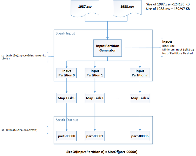
For example, If your source data is spread over 5 partitions, you have a parallelism of 5, and 5 files are created on the disk when Spark saves the result. Spark provides special functions to change the number of partitions like repartition and coalesce.
>>> df = spark.read.csv('retail_db/orders').repartition(4)
>>> df.rdd.getNumPartitions()
4
>>> df.write.csv('retail_db/orders_rep')
You can check the total blocks using the fsck command.
bash> hdfs fsck retail_db/orders_rep
 Total size:                   2999944 B
 Total dirs:                   1
 Total files:                  5
 Total symlinks:               0
 Total blocks (validated):     4 (avg. block size 749986 B)
 Minimally replicated blocks:  4 (100.0 %)
 Over-replicated blocks:       0 (0.0 %)
 Under-replicated blocks:      0 (0.0 %)
 Mis-replicated blocks:        0 (0.0 %)
 Default replication factor:   1
 Average block replication:    1.0
 Corrupt blocks:               0
 Missing replicas:             0 (0.0 %)
 Number of data-nodes:         2
 Number of racks:              1
Yarn Quick Preview
YARN is the component in Hadoop that coordinates Jobs, so that each Job has a fair share of the cluster’s resources. In certifications Spark typically runs in YARN mode. YARN consists of two daemon types:
- ResourceManager (RM) runs on master node, it allocates resources
- NodeManager (NM) runs on each worker nodes, it communicates with RM and manage node resources.
When a developers starts an application:
- ResourceManager allocates a container on one of the worker nodes and starts the ApplicationMaster in that container. Each application running has a single ApplicationMaster.
- ApplicationMaster calculates how many executors it needs to run the application and requests containers from the ResourceManager.
- ResourceManager tells the NodeManagers to allocate the requested number of containers, and then it passes the container information back to the ApplicationMaster.
- ApplicationMaster connects to NodeManagers, launching tasks and monitoring their progress. Each application tasks run in parallel.
YARN can run multiple applications at once.
Tune your Jobs in Apache Spark
By default Spark uses 2 executors with 1 GB RAM. With this configuration quite often you underutilize resources. You can change this configuration when you start PySpark.
bash> pyspark --master yarn --num-executors N --executors-cores C --executor-memory M
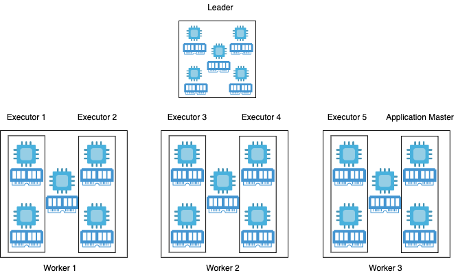
How to choose the value for N, C and M? You can use $ yarn top to get the cluster available cores and memory.

In this case you have a cluster with 3 workers node, the Memory is 18 GB and there are 15 VCores, each node has 5 VCores. If you assign one core per executor you will not be able to take advantage of running multiple tasks in the same JVM, if you use 5 cores per executor you will ends up with no resources for others demons processes.
So below you can find a step by step process:
- Leave 1 core per node for Hadoop/Yarn daemons, so the number of available cores per node is 5-1 = 4, the total available cores in the cluster is now 4*3 = 12.
- Based on the above considerations, let's use
--executor-core 2in this way you can take advantage of running multiple tasks in the same JVM. - You can obtain the number of available executors by using this formula [( total cores / num_cores_per_executor ) - 1]. In this formula, there is "minus one" because you need to leave one executor for the ApplicationManager.
- So the number of executors is
--num-executors 5that is the result of [(12 / 2)-1] = 5. - To set the Memory to use for each executor you need to consider also the ApplicationMaster, so in this case, it is equal to 18GB/6 = 3GB.
- By considering off heap overhead that is 7~10% of 3GB = 0.3GB. So, actual = 3GB - 0.3GB = 2.7GB
--executor-memory 2700M. Please note that 7~10% heap overhead is a kind of heuristic value.

By understanding memory settings and data size, you can accelerate the execution of jobs.
Setup Environment for Practice
To practice you need a Spark and Hadoop Environment, preferably with Hive support.
- Cloudera QuickStart VM: You can download the Virtual Machine from the Cloudera WebSite, the machine requires a login password. You can use The Download Page and The Login Credentials Page. I suggest to use this option if you have enough computational power on your local machine.
- If you have an Amazon Web Service Account you can use Elastic Map Reduce. This service let you to choose which framework to provide in the cluster, it is a fully managed service. I suggest to use this, or an equivalent service in Cloudera, if you want a real cluster experience. To cut-off the price of the cluster you can use EC2 Spot Instances, please refer to AWS Best Practice.
- You can use Vagrant Box with Hive and Spark.
- You can use Apache Zeppelin or local installation of PySpark.
Spark Quick Preview
Apache Spark, once part of the Hadoop ecosystem, is a fast and general engine for large-scale data processing. Tasks most frequently associated with Spark include ETL and SQL batch jobs, processing of streaming data and machine learning tasks. Spark provides two ways to write and run Spark code, in the Spark shell or as a free-standing application. The Spark shell is an interactive environment for Scala or Python.
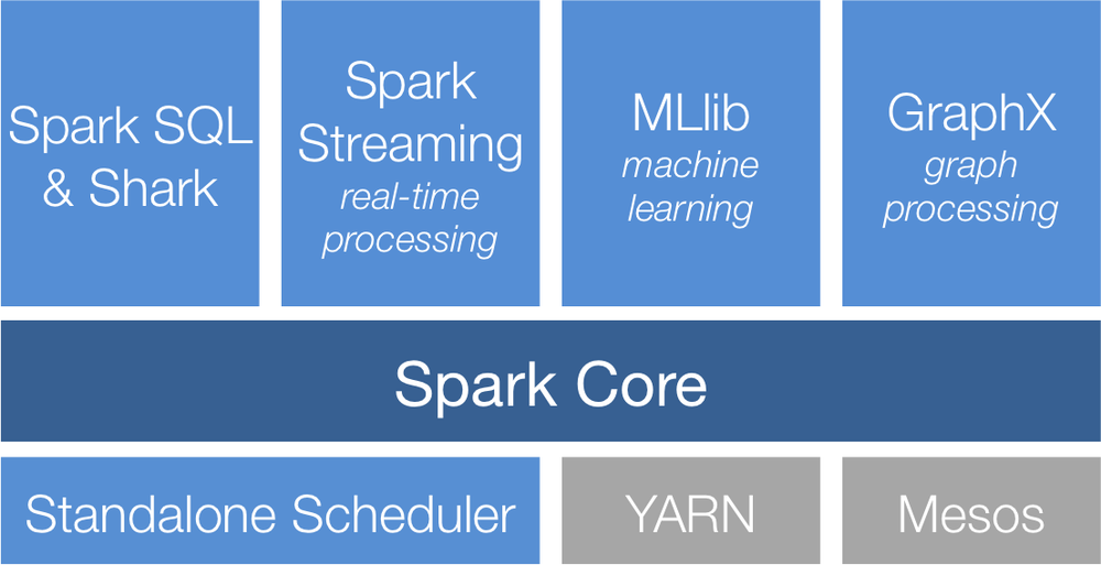
Apache Spark consists of a collection of APIs. The core Spark API provides resilient distributed datasets, or RDDs. All other Spark's APIs are built on top of the Spark Core. One of the key APIs in the Spark stack is Spark SQL, it is the main Spark entry point for working with structured data. The Spark machine learning library, which makes developing scalable machine learning applications. The Spark Streaming library provides an API to handle real-time data. Finally, GraphX is a library for graph-parallel computation.
Spark supports three different cluster platforms: Standalone, YARN, Mesos.
- Spark Standalone is a basic, easy-to-install cluster framework included with Spark.
$ pyspark --master localis helpful for limited uses, like learning or testing. - To use YARN, which is part of Apache Hadoop, simply set the master option to yarn
$ pyspark --master yarn, it provides full functionality. - Mesos is primarily intended to run non-Hadoop workloads, whereas YARN is geared mostly toward Hadoop.
$ pyspark mesos://masternode:port
Spark performs Distributed Computing, instead of processing on a single computer, a computationally-expensive execution is divided into many tasks that can be distributed between multiple computers that communicate with each other. Here you can see a change in the paradigm. In traditional systems, the data moves toward the processing unit, while in this case, the framework processes data where it is, and a coordinator distributes the application. Another difference is that instead of a Monolithic system, you have a Cluster made by a set of loosely or tightly connected computers that work together to behave as a single system. Each node performs the same task over Partitioned Data, the system distributes the data on multiple nodes, each one process its local data, everything is controlled and scheduled by software.
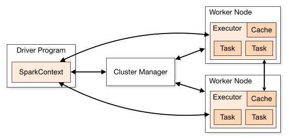
Spark applications run as independent sets of processes on a cluster, coordinated by the SparkContext object in your main program. It connect to Cluster Manager - local, YARN or Mesos - to allocate resources, once connected, Spark acquires executors and sends application code and finally SparkContext sends tasks to the executors to run. All Spark applications need to start with a SparkSession object.
The SparkSession class provides functions and attributes to access all of Spark functionality. Examples include
sql: execute a Spark SQL query, provides DataFrame and Dataset API.
- catalog: entry point for the Catalog API for managing tables.
- read: function to read data from a file or other data source.
- conf: object to manage Spark configuration settings.
- sparkContext: entry point for core Spark API, provides RDDs.
Spark shell automatically create a SparkSession object for you, otherwise you can create it using the following syntax.
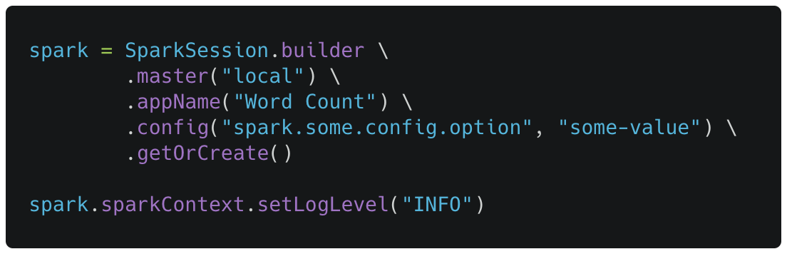
You can monitor a Spark application by using Spark UI, it displays useful information about the application like environment variables and executors information, memory usage, scheduler stages and tasks. This interface is running at http://<driver-node>:4040.
Spark is Fault-Tolerant, the distributed system can continue working properly even when a failure occurs.
Spark Core APIs
Resilient Distributed Datasets, or RDDs, are part of Spark Core, are immutable distributed collections of elements.
- Resilient: if data in memory is lost Spark can recreate the data using the RDD's lineage.
- Distributed: data is stored and processed on nodes throughout the cluster, tasks can be executed in parallel;
- Datasets: RDDs are an abstraction representing a set of data. Despite the name they are not actually based on the Spark SQL Dataset class.
The underlying data in RDDs can be unstructured, like text, or have some structure like JSON file, in both cases RDDs does not apply any schema. One important use of RDDs with Spark SQL is to convert unstructured or semi-structured data to the sort of structured data that DataFrames and Datasets were designed for.
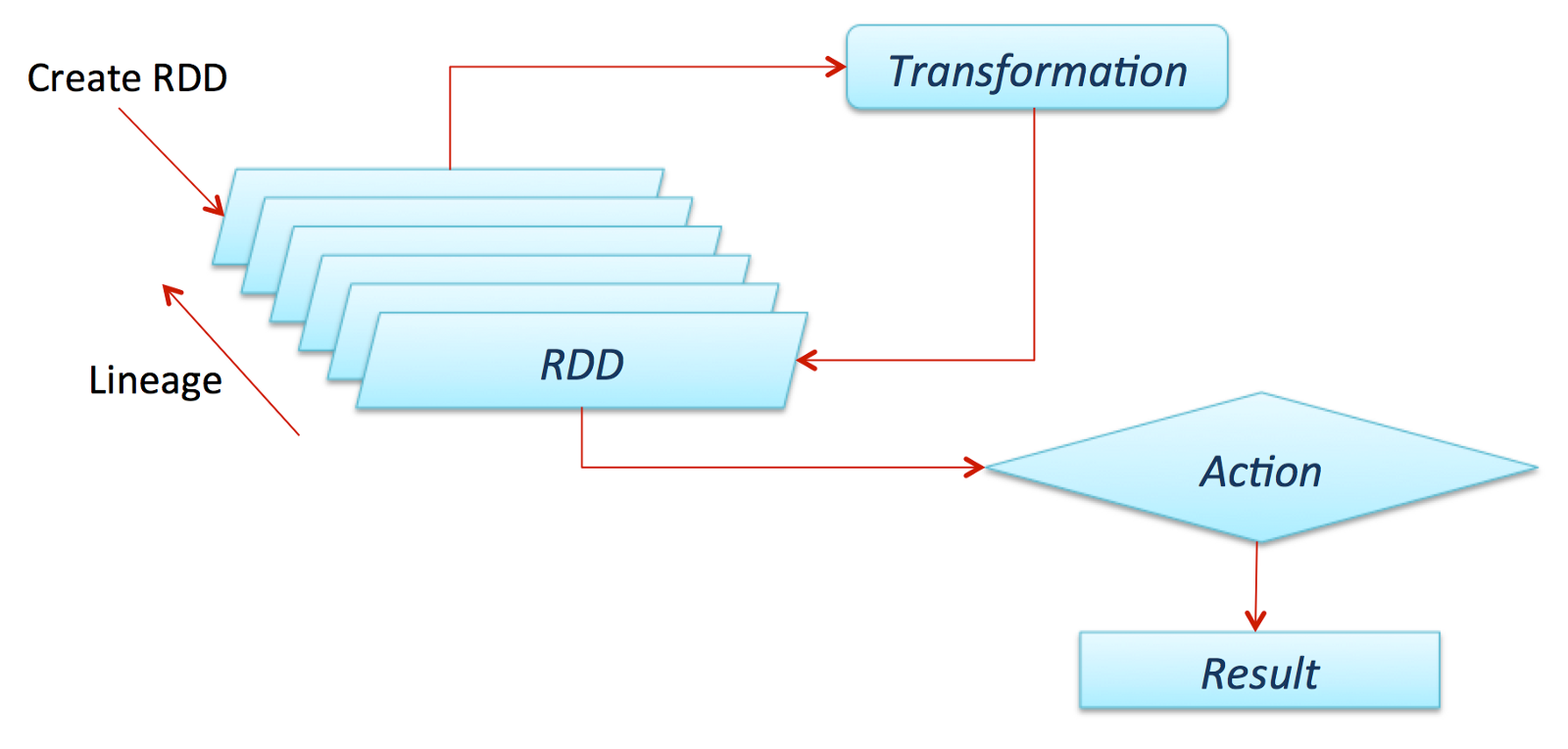
You can process and analyze data using a wide set of operations that can be categorized as either transformations or actions.
- Transformations are operations that create a new RDD as a result of performing some sort of transformation on the data in the original RDD. When a Spark application is running on a cluster, transformations are executed by the application’s executors in parallel, in JVMs distributed on worker nodes in the cluster.
- Actions are operations that generate output data from a RDD. Output from actions is typically either saved to a file or returned to the application’s driver process.
Transformations are lazy in nature, is an evaluation strategy which delays the evaluation of an expression until its value is needed. When you call some operation in RDD, Spark does not execute it immediately. Spark can keep track of the transformations of your data or lineage of the data during the jobs and efficiently minimizes the I/O by storing the Objects in memory, operations are executed by calling an action on data. Hence, in lazy evaluation data is not loaded until it is necessary.
The above code generate the following Spark DAG, where each Stage complete with a Shuffle operation. The Shuffle operation is used in Spark to re-distribute data across multiple partitions, it occurs when you have to run an operation on all elements of all partitions.
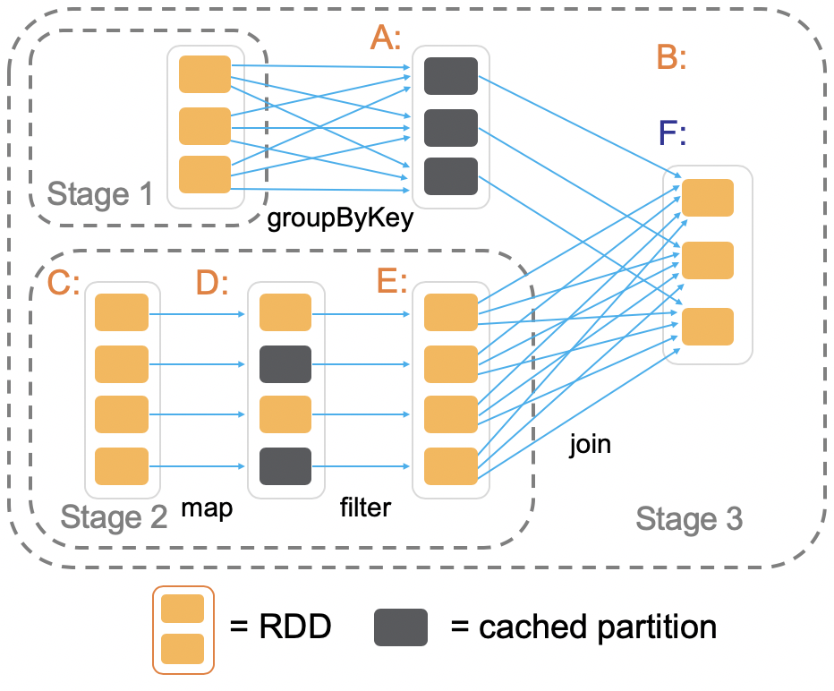
At the start there are two RDDs, order_rdd and customer_rdd. The order_rdd undergoes a groupByKey transformation which is stored as a cached partition, while customer_rdd undergoes two transformations: map and filter in stage 2. These two RDDs are then transformed into a third RDD using the join operation. For this job, Spark runs stage 2 and stage 3 while stage 1 is already in memory.
The action Take triggers the whole execution, the function is called with a value that specifies how many results to generate. Since data is not loaded until it is necessary, Spark load and process only data that is needed to provide the 10 results.
The method toDebugString provides a description of the RDD and its recursive execution for debugging.
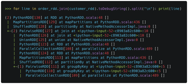
Lazy Evaluation considerations as also valid for both DataFrame and DataSets (only Scala). To generate debug string with DataFrame you can use Dataframe.explain a high-level operator that prints the execution plans to the console.
How to Create RDDs
You’ll need to use the Spark Context to work with RDDs, you can access to it using the sparkContext attribute of the session.
The Spark shell automatically assigns the Spark context to a variable called sc, so you can use that as well. The SparkContext class has a few functions to create new RDDs from files. You can obtain the functions list using dir(sc) or read the documentation of the functions using help(sc).
There are several types of data sources for RDDs:
- Files, including text files and other formats like json, csv, avro, etc.
- Data in memory, like list or others collections
- You can create RDDs from other RDDs
- you can create RDDs from Datasets and DataFrames by using the rdd property: DataFrames.rdd
flat/Map, filter
map(func)
Return a new distributed dataset which element are obtained by passing each element of the source through a function func.
flatMap(func)
Similar to map, but each input item can be mapped to 0 or more output items (so func should return a Sequence rather than a single item).
filter(func)
Return a new dataset formed by selecting those elements of the source on which func returns true.
Double RDDs
Double RDDs are a special type of RDDs that hold numerical data. Some of the functions that can be performed with Double RDDs are: distinct, sum, variance, mean, stats., etc.
Pair RDDs
Pair RDDs are a special form of RDD where each element must be a key/value pair, in other words a two-element tuple. The keys and the values can be of any type. The main use for pair RDDs is to execute transformations that use the map-reduce paradigm, and to perform operations like sorting, joining, and grouping data. Commonly used functions to create Pair RDDs are map, flatMap, flatMapValues and keyBy.
*ByKey, flat/mapValues
reduceByKey(func, [numPartitions])
Given a dataset of (K, V) pairs it returns a new dataset of (K, M) pairs where the values for each key are aggregated using the given reduce function: func. You can pass an optional argument numPartitions to set a different number of tasks. In the example, the function count how many times a word is in the source dataset.
mapValues(func)
This method maps the values while keeping the keys. It pass each value in the key-value pair RDD through a map function.
flatMapValues(func)
This method is a combination of flatMap and mapValues, like mapValues pass each value in the key-value pair RDD through a flatMap function without changing the keys, like flatMap the return is a Sequence rather than a single item. This method revert the operation groupByKey.
groupByKey([numPartitions])
Given a dataset of (K, V) pairs, returns a dataset of pairs (K, Iterable<V>). You can pass an optional argument numPartitions to set a different number of tasks. This method revert the flatMapValues operation.
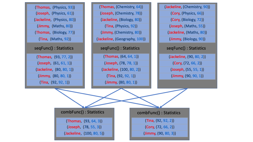
aggregateByKey(ZeroValue, seqFunc, combFunc, [numPartitions])
When called on a dataset of (K, V) pairs, returns a dataset of (K, U) pairs where the values for each key are aggregated using the given combine functions. This method takes as input:
- ZeroValue: defines the initial value of the aggregation and the shape.
- seqFunc: A combining function accepting two parameters and returns a single result. Initially, the function is called with the ZeroValue and the first item from the dataset. The method returns a result with ZeroValue shape. The function is then called again with the result obtained from previous step and the next value in the dataset. The second parameter keeps merging into the first parameter until there are items in the dataset. This function combines/merges values within a partition.
- combFunc: A merging function function accepting two parameters of ZeroValue shape generated by the seqFunc. In this case the parameters are merged into one. This step merges values across partitions.
In the example, seqFunc combines an item of zeroValue shape, a three elements tuple, with all items in a partition. The combFunc instead combines all the results from seqFunc, in this case both x and y have the same shape of the zeroValue.
foldByKey(ZeroValue, func, [numPartitions, partitionFunc])
Merges the values using the provided function. Unlike a traditional function fold over a list, the ZeroValue can be added an arbitrary number of times.
keyBy, lookup, count, sample
keyBy(func)
The keyBy transformation returns a new RDD in pair RDD form. The operation executes the passed function for each element to determine what the key for that element will be and pairs that with the whole input line as the value.
lookup(key)
This operation returns the list of values in the RDD for key, it is done efficiently if RDD is sorted by key.
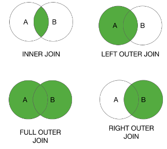
Join Operations
The join operation needs RDDs in Key/Value format. It generates a new Pair RDD that has the same Key and combined Values. Inner Join and Outer joins are supported through Join, leftOuterJoin, rightOuterJoin, and fullOuterJoin.
When called on datasets of type (K, V) and (K, W), returns a dataset of (K, (V, W)) pairs with all pairs of elements for each key.
join(otherDataset, [numPartitions])
leftOuterJoin(otherDataset, [numPartitions])
The left-join performs a join starting with the first (left-most) table. Then, any matched records from the second table (right-most) will be included. The right-join performs the same operation but starting with the second (right-most) table. The rightOuterJoin it is less used.
You can use left-join operation to obtain all element in first table that are not in the second table. As you can see in the above example, when there isn't a match between the tables all item in second table (left-join) are null.
fullOuterJoin(otherDataset, [numPartitions])
As you can see in the above example, all records that are not in the intersection between the two tables have null values.
Working with Sets
When you use set operations such as union and intersect, data should have a similar structure, both datasets should have the same columns.
You can also chain the set operators, for example when a union is performed, data will not be unique. You can use distinct to eliminate duplicates.
Sorting & Ranking
Ranking is very important in the process of decision making for any organization. Ranking can be classified as global as well as by key/group.
sortByKey([ascending], [numPartitions])
Given a dataset of (K, V) pairs, returns a dataset of (K, V) pairs. The sortByKey method sorts the RDD by a given key.
sortBy(keyfunc, ascending=True, numPartitions=None)
Given a dataset of (K, V) pairs, returns a dataset of (K, V) pairs. The sortBy method sorts this RDD by the given keyfunc. You can use the keyfunc the extract the key to use in sorting operation.
Since by default it sorts both keys in ascending order, if you want to change the sorting criteria for one key but not for the other you can use the negative numbers.
take(num)
Takes the first num elements of the RDD. You can use take to select top num elements from RDD.
takeOrdered(n, [ordering])
Get N elements from an RDD ordered in ascending order or as specified by the optional key function.
The methods takeOrdered and top are the same, the main difference is that in the method takeOrdered the ordering is performed in Ascending way by default, while in top method ordering is performed in Descending way by default.
Per-key or per-group ranking is one of the advanced transformations. Per-key or per-group ranking can be achieved having a good knowledge about how to manipulate collections. Usually the first step is to perform groupByKey, then you need to process the values as a collection using APIs of underlying programming language. Finally, invoke flatMap/flatMapValues. Let's have an example.
You have a dataset containing the students' names, the subject, and grade. Get the three highest grades for each subject, including duplicate grades. Sort the result by subject and then by grade.
In this example there are two functions:
- takewhile(predicate, iterable) - The function returns a takewhile object, it takes successive entries from an iterable as long as the predicate evaluates to true for each entry. Since it returns a takewhile object you must convert it to a list.
- sorted(iterable, key=None, reverse=False) - The function returns a new list containing all items from the iterable in ascending order. The function key can be supplied to customize the sort order, and the flag reverse can be set to request the result in descending order.
Saving data
To save data you must specify a path in HDFS, it must be a folder. Spark generates as many files as the number of partitions. You can get the current number of partitions using the getNumPartitions method, and you can change the number of partitions using repartition and coalesce.
getNumPartitions()
Returns the number of partitions in RDD
repartition(numPartitions)
Return a new RDD that has exactly numPartitions partitions. It can increase or decrease the level of parallelism in the RDD. Internally, it uses a shuffle to redistribute data. If you are decreasing the number of partitions in the RDD consider using coalesce which can avoid performing shuffle.
coalesce(numPartitions, shuffle=False)
The method returns a new RDD that is reduced into numPartitions partitions.
Save data into HDFS as field-delimited text
saveAsTextFile(path, compressionCodecClass=None)
Save the RDD as a text file, using string representations of elements.
You can use HDFS commands to check the result.
Save data into HDFS as JSON file
toDF(schema=None, sampleRatio=None)
Converts the current RDD into DataFrame, you can pass a schema or a list of column names.
You can use HDFS commands to check the result.
To be able to use toDF you have to create SQLContext (or SparkSession) first.
Retail Database
The later part of the course uses the retail_db database to provide some examples. The Cloudera team provides this database as part of its Big data developer training.
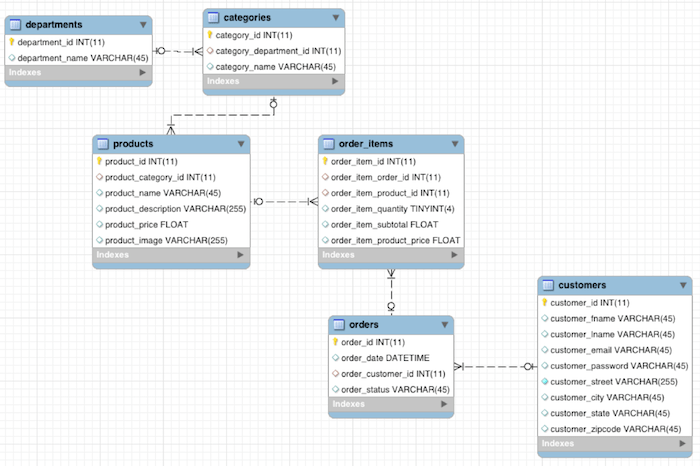
I have stored the database in Amazon S3 Bucket. You can download all files using the below links. The database has mainly six tables:
Hive APIs
The Apache Hive ™ data warehouse software facilitates reading, writing, and managing large datasets residing in distributed storage using SQL. Structure can be projected onto data already in storage. When you submit your HiveQL query, the Hive interpreter turns that query into either MapReduce or Spark jobs, and then it runs those on the cluster. Hive is a batch processing system. A lot of organizations still use Hive for ETL-type processes. You can use Hive DDL and DML statements to create database, tables and get data into tables.
Command Lines
One of the most immediate ways to use Hive is to start a command line console, there are two:
- Hive CLI, the original console which, although deprecated, is still available and can be convenient to experiment.
- Beeline, the current console, born to interact with HiveServer2, the updated version of the Hive server. Its connection to this service operates on JDBC.
To use the Hive CLI console the required command is as follows:
[hadoop@ip-172-31-40-195 ~]$ hive
hive>
A connection without options is ok for local access, or you can use the -h and -p options to specify the host you want to connect to and its TCP port.
There are three commands type:
- HiveQL to work with data.
- Shell commands using an exclamation mark “!”:
hive> !ls -la; - HDFS commands introduced by the dfs keyword:
hive> dfs -ls / ;
Beeline is the current console that should be preferred in production environments. You have to connect to an instance of HiveServer2 by providing connection string and login credentials. You can check the hive-site.xml configuration file for credentials.
$ beeline
Beeline version.. by Apache Hive
beeline> !connect jdbc:hive2://localhost:10000 <user> <pass>
...
Connected to: Apache Hive
...
The hive-site.xml configuration file is located in /etc/hive/conf, it contains all the Hive configuration properties. In this file the hive.metastore.warehouse.dir property defines the location of the default database for the Hive warehouse. Another way to get the property value is through the set command.
hive> SET hive.metastore.warehouse.dir;
hive.metastore.warehouse.dir=/user/hive/warehouse
Manage Databases
You can create a database with a create command and at least the name.
hive> CREATE DATABASE retail_db_txt;

hive> SHOW DATABASES;
default
retail_db_txt
However, aiming for greater completeness, you can write a definition like this:
hive> CREATE DATABASE IF NOT EXISTS retail_db_txt
COMMENT "To save orders informations"
WITH DBPROPERTIES ("author"="Giallo","scope"="revenue");
To have more detail yow can use the describe database command:
hive> DESCRIBE DATABASE EXTENDED retail_db_txt;
retail_db_txt To save orders informations hdfs://../retail_db_txt.db hadoop USER {author=Giallo, scope=revenue}
To select the current database you can use:
hive> USE retail_db_txt;
You can delete a database with the drop command, if you request to delete a non-existing database an error is returned that can be avoided with the if exists modifier:
hive> DROP DATABASE retail_db_txt;
hive> DROP DATABASE IF EXISTS not_exists_db;
Manage Tables
Once you have created a database, you can create and modify objects within it, for example you can create a table.
hive> CREATE TABLE orders (
  order_id int,
  order_date string,
  order_customer_id int,
  order_status string
)
row format delimited fields terminated by ","
STORED AS textfile;
The statement specifies, in addition to the name - orders - , three basic elements:
- Field names each defined with a given name and type,
- Saving format, in this case hive saves the data as text file,
- Delimiter to use in row parsing, the statement loads a CSV file.
We may also request detailed information about the table with the following command that provides statistics and structure details like fields name, data type, and information about the table:
hive> DESCRIBE FORMATTED orders;
OK
# col_name             data_type            comment

order_id             int
order_date           string
order_customer_id    int
order_status         string

# Detailed Table Information
Database:            default
Owner:               hadoop
CreateTime:          Sun Jul 19 23:24:34 UTC 2020
LastAccessTime:      UNKNOWN
Retention:           0
Location:            hdfs://.../orders
Table Type:          MANAGED_TABLE
Table Parameters:
 COLUMN_STATS_ACCURATE {\"BASIC_STATS\":\"true\"}
 numFiles             1
 numRows              3
 rawDataSize          65
 totalSize            68
 transient_lastDdlTime 1595202116

# Storage Information
SerDe Library:       org...hive.serde2.lazy.LazySimpleSerDe
InputFormat:         org.apache.hadoop.mapred.TextInputFormat
OutputFormat:        org...hive.ql.io.HiveIgnoreKeyTextOutputFormat
Compressed:          No
Num Buckets:         -1
Bucket Columns:      []
Sort Columns:        []
Storage Desc Params:
 field.delim          ,
 serialization.format ,
Time taken: 0.063 seconds, Fetched: 34 row(s)
Create external Table
Hive gives you the possibility to create external tables. An external table stores data in a folder other than the one that Hive uses as the default storage location. This is useful to incorporate external data into our work without making copies or moving it, but especially when data is shared with other applications pointing to the same storage.
hive> CREATE EXTERNAL TABLE orders (
  order_id int,
  order_date string,
  order_customer_id int,
  order_status string
)
row format delimited fields terminated by ","
stored as textfile
location "s3://gmucciolo.it/files/retail_db/orders/";

hive> CREATE EXTERNAL TABLE customers (
  customer_id int,
  customer_fname varchar(45),
  customer_lname varchar(45),
  customer_email varchar(45),
  customer_password varchar(45),
  customer_street varchar(45),
  customer_city varchar(45),
  customer_state varchar(45),
  customer_zipcode varchar(45)
)
row format delimited fields terminated by ','
stored as textfile
location "s3://gmucciolo.it/files/retail_db/customers/";
In this case the table points to an Amazon S3 location, be careful that the address must point to a folder, never to a file.
Create table by copying
You can create a table by copying the structure of another table.
hive> CREATE TABLE orders_copy LIKE orders;
You can use the command show to list all tables in the selected db
hive> SHOW TABLES;
orders
orders_copy
You can create a table by copying the data
hive> CREATE TABLE orders_copy AS SELECT * FROM orders;
Delete Table
You can completely delete the table by using the drop command.
hive> DROP TABLE orders_copy;
Manage data
If you want to insert three lines, you could invoke the following directive:
hive> INSERT INTO orders VALUES
(1, '2019-09-02', 5, 'COMPLETE'),
(2, '2019-11-03', 6, 'CLOSED'),
(3, '2019-12-17', 7, 'CLOSED');
Since you have both Hive and Hadoop, you can query the file system to print the current table content:
hive> dfs -cat /user/hive/warehouse/retail_db_txt.db/orders/000000_0;
1,2019-09-02,5,COMPLETE
2,2019-11-03,6,CLOSED
3,2019-12-17,7,CLOSED
You can massively import data from files in a table using the load data command.
hive> LOAD DATA LOCAL INPATH 'orders.csv' INTO TABLE orders;
With this command you are requesting:
- upload data ( LOAD DATA )
- from the local filesystem orders.csv file (LOCAL INPATH 'orders.csv')
- importing data into the transaction table (INTO TABLE transactions)
In this case file is in local path, deleting the LOCAL keyword Hive searches the file in HDFS. You can verify the success of the operation by invoking a query:
hive> SELECT * FROM orders LIMIT 10;

order_id order_date order_customer_id order_status
1  2013-07-25 00:00:00.0 11599 CLOSED
2  2013-07-25 00:00:00.0 256   PENDING_PAYMENT
3  2013-07-25 00:00:00.0 12111 COMPLETE
4  2013-07-25 00:00:00.0 8827  CLOSED
5  2013-07-25 00:00:00.0 11318 COMPLETE
6  2013-07-25 00:00:00.0 7130  COMPLETE
7  2013-07-25 00:00:00.0 4530  COMPLETE
8  2013-07-25 00:00:00.0 2911  PROCESSING
9  2013-07-25 00:00:00.0 5657  PENDING_PAYMENT
10 2013-07-25 00:00:00.0 5648  PENDING_PAYMENT
You can export data from a table to a path in HDFS.
hive> EXPORT TABLE retail_db_txt.orders TO '/tmp/orders';
Similarly, we can import all the files in a folder into a table.
hive> IMPORT TABLE retail_db_txt.orders FROM '/tmp/orders';
If you want to delete the whole data in a table you can use the truncate command
hive> TRUNCATE TABLE orders;
If you have a dataset in CSV format and you want to convert it to ORC, you can first upload the data into a table using the text format, and then copy the data to a new identical table using the ORC format.
hive> CREATE DATABASE retail_db_orc;
hive> USE retail_db_orc;
hive> CREATE TABLE orders (
  order_id int,
  order_date string,
  order_customer_id int,
  order_status string
)
stored as orc;

hive> INSERT INTO TABLE orders SELECT * FROM retail_db_txt.orders;
Partitions and Bucket
Partitioning a table is a way to organize it into partitions by dividing the table into different parts based on partition keys. This key will be based on the values of a particular field. You can use PARTITIONED BY to create a table. It creates folders with the name <field_name>=<field_value>.
The use of buckets instead involves a physical split of the data on disk into as fair portions as possible. You can use CLUSTERED BY (field_name) INTO num_bucket BUCKETS to create a table.
In order to achieve good performance, it is important to choose the most appropriate field in which to partition the data by adjusting it to the usual workload. It should always be a low cardinal attribute.
hive> CREATE TABLE orders_prt (order_id int, order_date string, order_customer_id int) PARTITIONED BY (order_status string COMMENT 'Order State') STORED AS ORC;

hive> describe orders_prt;
order_id             int
order_date           timestamp
order_customer_id    int
order_status         string               Order State
# Partition Information
# col_name           data_type            comment
order_status         string               Order State

hive> SET hive.exec.dynamic.partition.mode=nonstrict;
hive> INSERT OVERWRITE TABLE orders_prt PARTITION(order_status) SELECT * FROM orders;
As you can see there is the keyword PARTITIONED BY followed by a pair of round brackets in which there is the field that contains the distinctive values of the individual partitions. One of the possible ways to populate a partitioned table is by using an INSERT operation, but you have to make sure to enable the nonstrict mode. This will allow dynamic activation of the partitions.
hive> dfs -ls /user/hive/warehouse/orders_prt;
Found 9 items
drwxr-xr-t   ..../orders_prt/order_status=CANCELED
drwxr-xr-t   ..../orders_prt/order_status=CLOSED
drwxr-xr-t   ..../orders_prt/order_status=COMPLETE
drwxr-xr-t   ..../orders_prt/order_status=ON_HOLD
drwxr-xr-t   ..../orders_prt/order_status=PAYMENT_REVIEW
drwxr-xr-t   ..../orders_prt/order_status=PENDING
drwxr-xr-t   ..../orders_prt/order_status=PENDING_PAYMENT
drwxr-xr-t   ..../orders_prt/order_status=PROCESSING
drwxr-xr-t   ..../orders_prt/order_status=SUSPECTED_FRAUD
Exactly there is a folder for every possible value in the order_status field: this means partitioning the data.
While Hive partition creates a separate directory for a column(s) value, Bucketing decomposes data into more manageable or equal parts. With partitioning, there is a possibility that you can create multiple small partitions based on column values. If you go for bucketing, you are restricting number of buckets to store the data. This number is defined during table creation scripts.
hive> CREATE TABLE orders_bkt (order_id int, order_date timestamp, order_customer_id int, order_status varchar(45) ) CLUSTERED BY (order_status) INTO 9 BUCKETS STORED AS ORC;

hive> describe orders_bkt;
order_id             int
order_date           timestamp
order_customer_id    int
order_status         string

hive> INSERT INTO TABLE orders_bkt SELECT * FROM orders;
As you can see there is the keyword CLUSTERED BY followed by a pair of round brackets in which there is the field that contains the filed to use in bucketing and then the number of buckets to generate. You can directly perform INSERT operation in thi case.
hive> dfs -ls /user/hive/warehouse/orders_bkt;
Found 6 items
-rwxr-xr-t   ..../orders_bkt/000001_0
-rwxr-xr-t   ..../orders_bkt/000002_0
-rwxr-xr-t   ..../orders_bkt/000003_0
-rwxr-xr-t   ..../orders_bkt/000004_0
-rwxr-xr-t   ..../orders_bkt/000006_0
-rwxr-xr-t   ..../orders_bkt/000007_0
Hive Functions
You can obtain thee complete list of built-in functions easily. Hive gives you the possibility to check the function's documentation by using the command "describe" and even more information using the option "extended".
SHOW FUNCTIONS;
DESCRIBE FUNCTION <function_name>;
DESCRIBE FUNCTION EXTENDED <function_name>;
Below you can find the main Hive functions.
hive> DESCRIBE FUNCTION abs;
abs(x) - returns the absolute value of x

hive> DESCRIBE FUNCTION EXTENDED abs;
abs(x) - returns the absolute value of x
Example:
  > SELECT abs(0) FROM src LIMIT 1;
  0
  > SELECT abs(-5) FROM src LIMIT 1;
  5
Strings Functions
- substring(str, pos[, len]) or substr(str, pos[, len]) - returns the substring of str that starts at pos and is of length len. You can also use negative indexes, in this case, the function starts to count from the end of the string.
hive> SELECT order_id, substr(order_date, 1, 10), order_customer_id, order_status FROM orders LIMIT 5;

order_id order_date order_customer_id order_status
1 2013-07-25 11599 CLOSED
2 2013-07-25 256   PENDING_PAYMENT
3 2013-07-25 12111 COMPLETE
4 2013-07-25 8827  CLOSED
5 2013-07-25 11318 COMPLETE

hive> SELECT substr('Hello World', -5);
World
- instr(str, substr) - Returns the index of the first occurance of substr in str
hive> SELECT instr('Hello World', 'World');
7- like(str, pattern) - Checks if str matches pattern
hive> SELECT * FROM orders WHERE order_status LIKE "C%" LIMIT 5;

order_id order_date order_customer_id order_status
1 2013-07-25 00:00:00.0 11599 CLOSED
3 2013-07-25 00:00:00.0 12111 COMPLETE
4 2013-07-25 00:00:00.0 8827  CLOSED
5 2013-07-25 00:00:00.0 11318 COMPLETE
6 2013-07-25 00:00:00.0 7130  COMPLETE

hive> SELECT 'Hello World' like 'Hello%';
true
hive> SELECT 'Hello World' like 'Hi%';
false
- rlike(str, regexp) - Returns true if str matches regexp and false otherwise
hive> SELECT * FROM orders WHERE order_status RLIKE "CLOSED|COMPLETE" LIMIT 5;

order_id order_date order_customer_id order_status
1 2013-07-25 00:00:00.0 11599 CLOSED
3 2013-07-25 00:00:00.0 12111 COMPLETE
4 2013-07-25 00:00:00.0 8827  CLOSED
5 2013-07-25 00:00:00.0 11318 COMPLETE
6 2013-07-25 00:00:00.0 7130  COMPLETE

hive> SELECT 'Hello World' RLIKE '[A-Z]{1}[a-z]*';
true
hive> SELECT 'hello world' RLIKE '[A-Z]{1}[a-z]*';
false
- length(str | binary) - Returns the length of str or number of bytes in binary data
hive>SELECT length('Hello World');
11

hive>SELECT DISTINCT order_status, length(order_status) FROM orders;

order_status      length(order_status)
CANCELED          8
COMPLETE          8
ON_HOLD           7
PAYMENT_REVIEW    14
PENDING           7
SUSPECTED_FRAUD   15
CLOSED            6
PENDING_PAYMENT   15
PROCESSING 10- lcase(str) or lower(str) - Returns str with all characters changed to lowercase
hive>SELECT lcase('Hello World');
hello world- ucase(str) or upper(str) - Returns str with all characters changed to uppercase
hive>SELECT ucase('Hello World');
HELLO WORLD- lpad(str, len, pad) - Returns str, left-padded with pad to a length of len. rpad(str, len, pad) - Returns str, right-padded with pad to a length of len. In this example 5 is the maximum length of order_customer_id while 15 is the maximum length of order_status. If the len value is less than the current length the string is truncated.
hive> SELECT order_id, rpad(order_date, 10, '_') AS pad_od, lpad(order_customer_id, 5, 0) AS pad_cid, rpad(order_status, 15, '_') AS pad_os FROM orders LIMIT 5;

order_id  pad_od      pad_cid  pad_os
1         2013-07-25  11599    CLOSED_________
2         2013-07-25  00256    PENDING_PAYMENT
3         2013-07-25  12111    COMPLETE_______
4         2013-07-25  08827    CLOSED_________
5         2013-07-25  11318    COMPLETE_______
- concat(str1, str2, ... strN) - returns the concatenation of str1, str2, ... strN, if you provide binary data it returns the concatenation of bytes in binary.
hive> SELECT concat('Hello', ',', 'Nice', ',', 'World');
Hello,Nice,World

hive> SELECT customer_fname, customer_lname, substr(customer_lname,1,2)||substr(customer_fname,1,1) AS trigram FROM customers LIMIT 5;

customer_fname customer_lname trigram
Mary           Barrett        BaM
Ann            Smith          SmA
Mary           Jones          JoM
Robert Hudson HuR- concat_ws(separator, [string | array(string)]+) - returns the concatenation of the strings separated by the separator.
hive> SELECT concat_ws(',', 'Hello', 'Nice', 'Hi');
Hello,Nice,Hi- split(str, regex) - Splits string using occurrences that match regex
hive> SELECT split('Hello,Nice,Hi', ',');
["Hello","Nice","Hi"]- explode(a) - separates the elements of array a into multiple rows, or the elements of a map into multiple rows and columns
hive> SELECT explode(split('Hello,Nice,Hi', ','));
Hello
Nice
Hi

hive> SELECT tf1.*, t.*, tf2.*
      FROM (SELECT 'World') t
      LATERAL VIEW explode(split('Hello,Nice,Hi', ',')) tf1;

Hello World
Nice  World
Hi World- trim(str) - Removes the leading and trailing space characters from str. ltrim(str) - Removes the leading space characters from str. rtrim(str) - Removes the trailing space characters from str.
hive> SELECT trim('  both_   ')||rtrim('are_    ')||ltrim('  ok');
both_are_ok- initcap(str) - Returns str, with the first letter of each word in uppercase, all other letters in lowercase. Words are delimited by white space.
hive> SELECT initcap('hELLO wORLD');
Hello World

hive> SELECT DISTINCT initcap(order_status) FROM orders;

Closed
Payment_review
Pending_payment
Canceled
Complete
On_hold
Pending
Processing
Suspected_fraud
Date Functions
In Hive you can manipulate dates, there are many built-in functions you can use. Among the many available you have current_date and current_timestamp. The first one returns the current date at the start of query evaluation, while the second one returns the current timestamp. Those two are very useful when you are comparing dates.
hive> SELECT current_date;
2020-07-30
hive> SELECT current_timestamp;
2020-07-30 19:25:12.186
- date_add(start_date, num_days) - Returns the date that is num_days after start_date.
hive> SELECT date_add(current_date, 39);
2020-09-07
- date_sub(start_date, num_days) - Returns the date that is num_days before start_date.
hive> SELECT date_sub(current_date, 39);
2020-06-21
- to_unix_timestamp(date[, pattern]) - Returns the UNIX timestamp, it converts the specified time to number of seconds since 1970-01-01.
hive>SELECT to_unix_timestamp("2020/07/30 07:25:12.186 PM", "yyyy/MM/dd hh:mm:ss.SSS aa");
1596137112- from_unixtime(unix_time, format) - returns unix_time in the specified format. As you can see in this operations you lost milliseconds.
hive>SELECT from_unixtime(1596137112, "yyyy/MM/dd hh:mm:ss.SSS aa")
2020/07/30 07:25:12.000 PM
- date_format(date/timestamp/string, fmt) - converts a date/timestamp/string to a value of string in the format specified by the date format fmt. You can apply this function to a date column or a string parsable as a date. The pattern value of the first argument can not be arbitrary. The pattern you can provide should be like this 'yyyy-MM-dd' or 'yyyy-MM-dd HH:mm:ss', basically the same you get from current_date and current_timestamp. If you have a string column with a non-standard format, you must first convert it to a pattern suitable for the to_date using to_unix_timestamp and then from_unix_time.
hive>SELECT date_format('2020-07-30 19:25:12', 'yyyy');
2020

hive>SELECT from_unixtime(to_unix_timestamp("07/30/2020 07:25:12 PM","MM/dd/yyyy hh:mm:ss aa"),"yyyy-MM-dd HH:mm:ss");
2020-07-30 19:25:12

hive>SELECT date_format('2020-07-30 19:25:12', 'W');
5 # Week In Month
hive>SELECT date_format('2020-07-30 19:25:12', 'w');
31 # Week In Year
hive>SELECT date_format('2020-07-30 19:25:12', 'D');
212 # Day in year
Supported formats are SimpleDateFormat. You can use also functions like:
- weekofyear(date) - Returns the week of the year of the given date
- dayofweek(param) - Returns the day of the week of date/timestamp
- day(param) - Returns the day of the month of date/timestamp, or day component of interval, it is the same as dayofmonth(param)
hive>SELECT day('2020-07-30');
30

hive>SELECT day(date_add(current_date, 40) - current_date);
40- datediff(date1, date2) - Returns the number of days between date1 and date2
hive>SELECT datediff(date_add(current_date, 1095) - current_date);
- year(param) - Returns the year component of the date/timestamp/interval
- month(param) - Returns the month component of the date/timestamp/interval
- minute(param) - Returns the minute component of the string/timestamp/interval
hive>SELECT year('2020-07-30');
2020

interval?- to_date(date/timestamp/string) - Extracts the date part of the date, timestamp or string.
hive> SELECT to_date('2020-07-30 19:25:12');
2020-07-30- next_day(start_date, day_of_week/em>) - Returns the first date which is later than start_date and named as indicated.
hive>SELECT next_day('2020-07-30', 'MONDAY');
2020-08-03- months_between(date1, date2, roundOff) - returns number of months between dates date1 and date2. It also calculates the fractional portion of the result based on a 31-day month. The result is rounded to 8 decimal places by default. Set roundOff=false otherwise. It performs date1 - date2 operation.
hive>SELECT months_between(date_add(current_date, 1095), current_date);
36.0

hive>SELECT months_between(date_sub(current_date, 15), current_date);
-0.48387097

hive>SELECT months_between(date_add(current_date, 15), current_date);
0.48387097
- to_utc_timestamp(timestamp, string timezone) - Assumes given timestamp is in given timezone and converts to UTC
hive> SELECT to_utc_timestamp(current_timestamp, "2");
2020-07-30 21:26:58.902
- from_utc_timestamp(timestamp, string timezone) - Assumes given timestamp is UTC and converts to given timezone
hive> SELECT to_utc_timestamp("2020-07-30 21:26:58.902", "2");
2020-07-30 21:26:58.902
Aggregation Functions
Among the most common functions used in queries are aggregation functions that provide results from data in the fields of a table.
- count(*) - Returns the total number of retrieved rows
hive>SELECT count(*) FROM orders;
68883

hive>SELECT count(*) FROM customers;
12435
- sum(x) - Returns the sum of a set of numbers
- min(x) - Returns the min of a set of numbers
- max(x) - Returns the maximum of a set of numbers
- avg(x) - Returns the mean of a set of numbers
- round(x[, d]) - round x to d decimal places
hive>SELECT round(sum(order_item_subtotal),2), min(order_item_subtotal), max(order_item_subtotal), round(avg(order_item_subtotal),2) FROM order_items;

sum           min  max     avg
3.432261993E7 9.99 1999.99 199.32
Conditional Functions
With IF we can evaluate a condition and define which value will be returned if it is TRUE and which if not.
hive> SELECT *, IF(order_status rlike "CLOSED|COMPLETE", "DONE", "WIP") AS agg_status FROM orders LIMIT 10;

order_id order_date order_customer_id order_status agg_status
1  2013-07-25 00:00:00.0 11599 CLOSED          DONE
2  2013-07-25 00:00:00.0 256   PENDING_PAYMENT WIP
3  2013-07-25 00:00:00.0 12111 COMPLETE        DONE
4  2013-07-25 00:00:00.0 8827  CLOSED          DONE
5  2013-07-25 00:00:00.0 11318 COMPLETE        DONE
6  2013-07-25 00:00:00.0 7130  COMPLETE        DONE
7  2013-07-25 00:00:00.0 4530  COMPLETE        DONE
8  2013-07-25 00:00:00.0 2911  PROCESSING      WIP
9  2013-07-25 00:00:00.0 5657  PENDING_PAYMENT WIP
10 2013-07-25 00:00:00.0 5648  PENDING_PAYMENT WIP
When you need to provide specific values you can use the construct CASE...WHEN...THEN...END. With CASE you can specify the name of a field and with the blocks WHEN...THEN (you can repeat them several times) you indicate which value must be returned in correspondence to a certain data in the field. At the end you report an END to close the block. If a default possibility exists, it can be introduced with the ELSE keyword at the end of the sequence WHEN...THEN.
hive>SELECT *,
CASE order_status
WHEN "CLOSED" THEN "DONE"
WHEN "COMPLETE" THEN "DONE"
ELSE "WIP"
END FROM orders LIMIT 10;

order_id order_date order_customer_id order_status agg_status
1 2013-07-25 00:00:00.0 11599 CLOSED          DONE
...
2 2013-07-25 00:00:00.0 256   PENDING_PAYMENT WIP

hive> SELECT *,
CASE
WHEN order_status IN ("CLOSED", "COMPLETE") THEN "DONE"
WHEN order_status IN ("CANCELED", "SUSPECTED_FRAUD") THEN "ERROR"
ELSE "WIP"
END FROM orders LIMIT 5;

order_id order_date order_customer_id order_status agg_status
1  2013-07-25 00:00:00.0 11599 CLOSED          DONE
2  2013-07-25 00:00:00.0 256   PENDING_PAYMENT WIP
...
50 2013-07-25 00:00:00.0 5225  CANCELED        ERROR
...
69 2013-07-25 00:00:00.0 2821  SUSPECTED_FRAUD ERROR

hive>SELECT *,
CASE
WHEN order_status LIKE "%MPLE%" THEN "DONE"
END FROM orders LIMIT 10;

order_id order_date order_customer_id order_status is_done
1 2013-07-25 00:00:00.0 11599 CLOSED          NULL
2 2013-07-25 00:00:00.0 256   PENDING_PAYMENT NULL
3 2013-07-25 00:00:00.0 12111 COMPLETE        DONE
...
- nvl(value,default_value) - Returns default value if value is null else returns value
hive> SELECT * FROM ( SELECT *, nvl(order_status, 'UNK') as order_status FROM orders ) as T WHERE T.order_status = 'UNK' LIMIT 10;
The select does not return any results, there are no orders with unknown status.
Grouping, Sorting and Filtering
This section is about how to sort and group data. The sort operation allows you to obtain the results in a specific order based on the value of one or more fields. The group operation allows you to divide in groups the records identified thanks to the values present in certain fields, possibly processed with functions. The filter operation allows you to select which record to provide in the final result.
All the examples will refer to the retail_db dataset.
Sorting: Order By, Sort By, Distribute By, Cluster By
The sorting is done by means of the ORDER BY clause which requires the indication of at least one field on the basis of which to sort the results. By default the sorting is done in an ascending order.
hive> SELECT * FROM orders ORDER BY order_id LIMIT 5;

order_id order_date order_customer_id order_status
1 2013-07-25 00:00:00.0 11599 CLOSED
2 2013-07-25 00:00:00.0 256   PENDING_PAYMENT
3 2013-07-25 00:00:00.0 12111 COMPLETE
4 2013-07-25 00:00:00.0 8827  CLOSED
5 2013-07-25 00:00:00.0 11318 COMPLETE
To get the results in reverse order you will need to specify the DESC keyword.
hive> SELECT * FROM orders ORDER BY order_id DESC LIMIT 5;

order_id order_date order_customer_id order_status
68883 2014-07-23 00:00:00.0 5533  COMPLETE
68882 2014-07-22 00:00:00.0 10000 ON_HOLD
68881 2014-07-19 00:00:00.0 2518  PENDING_PAYMENT
68880 2014-07-13 00:00:00.0 1117  COMPLETE
68879 2014-07-09 00:00:00.0 778   COMPLETE
You can provide many values to ORDER BY clause, in this case sorting is performed with priority. You get the results in descending order by order_customer_id, then by order_id in ascending order.
hive> SELECT * FROM orders ORDER BY order_customer_id DESC, order_id ASC LIMIT 6;

order_id order_date order_customer_id order_status
22945 2013-12-13 00:00:00.0 1 COMPLETE
67863 2013-11-30 00:00:00.0 2 COMPLETE
57963 2013-08-02 00:00:00.0 2 ON_HOLD
33865 2014-02-18 00:00:00.0 2 COMPLETE
15192 2013-10-29 00:00:00.0 2 PENDING_PAYMENT
61453 2013-12-14 00:00:00.0 3 COMPLETE
Hive support SORT BY, DISTRIBUTE BY and CLUSTER BY.
Lets see the differences. First of all you need to create a sample data.
bash> echo -e "19\n0\n1\n3\n2\n17\n4\n5\n7\n14\n6\n8\n9" > data.txt
Then you need to create a sample table and load the data.
hive> CREATE TABLE sample (val int);
hive> SET mapred.reduce.tasks=2; # MAX 2 reduce tasks
hive> LOAD DATA LOCAL INPATH 'data.txt' INTO TABLE sample;
You can query the table to verify that the initial order is the same of the data.txt file.
- ORDER BY x: guarantees global ordering, but does this by pushing all data through just one reducer. This is basically unacceptable for large datasets. You end up one sorted file as output.
hive> SELECT * FROM sample ORDER BY val;
0,1,2,3,4,5,6,7,8,9,14,17,19
- SORT BY x: orders data at each of N reducers, but each reducer can receive overlapping ranges of data. You can end up with N or more sorted files with overlapping ranges. It performs local sorting.
hive> SELECT * FROM sample SORT BY val;
1,2,3,5,6,8,9,14,19,0,4,7,17
- DISTRIBUTE BY x: ensures each of N reducers gets non-overlapping ranges of x, but doesn't sort the output of each reducer. You end up with N or more unsorted files with non-overlapping ranges. It does NOT sort data.
hive> SELECT * FROM sample DISTRIBUTE BY val;
8,6,14,4,2,0,9,7,5,17,3,1,19
- CLUSTER BY x: ensures each of N reducers gets non-overlapping ranges, then sorts by those ranges at the reducers. It is a short-cut for DISTRIBUTE BY x and SORT BY x. It performs local sorting.
hive> SELECT * FROM sample CLUSTER BY val;
0,2,4,6,8,14,1,3,5,7,9,17,19
So, to perform local sorting you can use DISTRIBUTE BY clause together with SORT BY clause when you need to sort many columns, while you can use CLUSTER BY if you distribute and sort using same column.
hive> SELECT * FROM orders DISTRIBUTE BY order_customer_id SORT BY order_customer_id, order_id LIMIT 10;
Grouping: Group By
The GROUP BY clause is used to perform grouping, also followed by the fields under which we want to group. Grouping essentially means dividing records into different groups, each of which is marked by the same values in the fields indicated by GROUP BY. For example, below you can see the total number of orders for each status.
hive> SELECT order_status, count(*) FROM orders GROUP BY order_status;

order_status    count
CLOSED          7556
COMPLETE        22899
PENDING         7610
SUSPECTED_FRAUD 1558
CANCELED        1428
ON_HOLD         3798
PAYMENT_REVIEW  729
PENDING_PAYMENT 15030
PROCESSING      8275
If you want to see the proposed lines deployed in descending order you can apply an ORDER BY. Note, you have to use an alias applied to the function COUNT(*):
hive> SELECT order_status, count(*) AS order_count FROM orders GROUP BY order_status ORDER BY order_count DESC;

order_status    count
COMPLETE        22899
PENDING_PAYMENT 15030
PROCESSING      8275
PENDING         7610
CLOSED          7556
ON_HOLD         3798
SUSPECTED_FRAUD 1558
CANCELED        1428
PAYMENT_REVIEW  729
You cannot use GROUP BY clause with columns created in the current query.
Filtering: Where, Having
In Hive, you can use where and having to filter your data. Both work similarly to a condition. You can use where and having to filter the data using the condition and gives you a result. The main difference between the two is:
- WHERE: is used to fetch data (rows) from the table. Data that doesn't pass the condition will not be into the result.
- HAVING: is later used to filter summarized data or grouped data.
hive> SELECT * FROM orders WHERE order_status IN ('COMPLETE','CLOSED') LIMIT 5;

order_id order_date order_customer_id order_status
1 2013-07-25 00:00:00.0 11599  CLOSED
3 2013-07-25 00:00:00.0 12111  COMPLETE
4 2013-07-25 00:00:00.0 8827   CLOSED
5 2013-07-25 00:00:00.0 11318  COMPLETE
6 2013-07-25 00:00:00.0 7130   COMPLETE

hive> SELECT order_status, count(*) AS order_count FROM orders GROUP BY order_status HAVING order_count > 8000;

order_status    order_count
PENDING_PAYMENT 15030
COMPLETE        22899
PROCESSING      8275

hive> SELECT order_status, count(*) AS order_count FROM orders WHERE order_status IN ('COMPLETE','CLOSED') GROUP BY order_status HAVING order_count > 8000;

order_status order_count
COMPLETE     22899
In latter query Hive performs: where-filtering, group by operation, count aggregation and finally having-filtering. Exactly in this order.
Cast Operations
Hive CAST function converts the value of an expression to any other type. The result of the function will be NULL in case if function cannot converts to particular data type. The syntax is CAST (<from-type> AS <to-type>) from-type & to-type could be any data type. Please find below some very easy examples.
hive> SELECT CAST('10' AS int); # 10
hive> SELECT CAST(10 AS string); # 10
hive> SELECT cast('2018-06-05' AS DATE); # 2018-06-05
You can describe order table to see columns and types, order_date is a string.
hive> DESCRIBE orders;
order_id             int
order_date           string
order_customer_id    int
order_status         string
hive> SELECT *, CAST(order_date AS DATE) AS c_order_date FROM orders LIMIT 1;

order_id order_date order_customer_id order_status c_order_date
1 2013-07-25 00:00:00.0 11599 CLOSED 2013-07-25
To cast order_date you can clone the table by select
hive> CREATE TABLE orders_date STORED AS PARQUET AS SELECT order_id, CAST(order_date AS TIMESTAMP), order_customer_id, order_status FROM orders;

hive> DESCRIBE orders_data;
order_id             int
order_date           timestamp
order_customer_id    int
order_status         string

hive> SELECT * FROM orders_data LIMIT 1;
1 2013-07-25 00:00:00.0 11599 CLOSED
Working with Sets
Hadoop Hive supports following set operators.
- UNION: combines the results of two or more similar sub-queries into a single result set that contains the rows that are returned by all SELECT statements. Data types of the column should match. It Removes duplicate rows from the result set.
- UNION ALL: combines the results of two or more similar sub-queries into a single result set. Data types of the column should match. It does NOT remove duplicate rows from the result set.
hive> SELECT 1, "Hello" UNION ALL SELECT 1, "World" UNION ALL SELECT 2, "Hello" UNION ALL SELECT 1, "World";
1 Hello
1 World
2 Hello
1 World

hive> SELECT 1, "Hello" UNION  SELECT 1, "World" UNION  SELECT 2, "Hello" UNION SELECT 1, "World";
2 Hello
1 Hello
1 World
Joins Operations
The Join mechanism is central in the use of relational databases: it allows to align tables and extract their value by leveraging on relationships. With Join's operations you are able to carry out analyses involving several tables.
You can use the relation between orders and order_items to obtain for each order: the date, the customer id, the products id, subtotal and status.
hive> CREATE EXTERNAL TABLE order_items (order_item_id int, order_item_order_id int, order_item_product_id int, order_item_quantity int, order_item_subtotal float, order_item_product_price float) row format delimited fields terminated by ',' stored as textfile location "s3://gmucciolo.it/files/retail_db/order_items";

hive> SELECT o.order_id, oi.order_item_id, oi.order_item_subtotal, CAST(o.order_date AS DATE), o.order_status FROM orders AS o
JOIN order_items AS oi ON order_id = order_item_order_id
LIMIT 10;

order_id order_item_id order_item_subtotal order_date order_status
1 1  299.98  2013-07-25 CLOSED
2 2  199.99  2013-07-25 PENDING_PAYMENT
2 3  250.0   2013-07-25 PENDING_PAYMENT
2 4  129.99  2013-07-25 PENDING_PAYMENT
4 5  49.98   2013-07-25 CLOSED
4 6  299.95  2013-07-25 CLOSED
4 7  150.0   2013-07-25 CLOSED
4 8  199.92  2013-07-25 CLOSED
5 9  299.98  2013-07-25 COMPLETE
5 10 299.95  2013-07-25 COMPLETE
You'll get the above lines. The statement uses a pure Join that returns only the rows on which there is a match between the two tables. In addition to the word JOIN the fundamental point is ON which introduces the condition that determines how the fields cross each other. You may need to use aliases to avoid conflicts between fields with the same name. You can also use multiple concatenated JOINs to take advantage of all available tables.
hive> SELECT o.order_id, oi.order_item_id, oi.order_item_subtotal, CAST(o.order_date AS DATE), o.order_status, c.customer_fname, c.customer_lname
FROM orders AS o
JOIN order_items AS oi ON order_id = order_item_order_id
JOIN customers AS c ON order_customer_id = customer_id
LIMIT 10;

1 1  299.98  2013-07-25 CLOSED          Mary Malone
2 2  199.99  2013-07-25 PENDING_PAYMENT David Rodriguez
2 3  250.0   2013-07-25 PENDING_PAYMENT David Rodriguez
2 4  129.99  2013-07-25 PENDING_PAYMENT David Rodriguez
4 5  49.98   2013-07-25 CLOSED          Brian Wilson
4 6  299.95  2013-07-25 CLOSED          Brian Wilson
4 7  150.0   2013-07-25 CLOSED          Brian Wilson
4 8  199.92  2013-07-25 CLOSED          Brian Wilson
5 9  299.98  2013-07-25 COMPLETE        Mary Henry
5 10 299.95  2013-07-25 COMPLETE        Mary Henry
In this case we get lines where we also have the name and surname of the person who placed the order.
Asymmetric Joins
You can perform asymmetric JOINs by applying the LEFT keyword to the JOIN, in this case you require that all the records in the table on the left of the JOIN must be expressed, those in the other table will be linked only if an exact match occurs.
hive> SELECT c.customer_id, o.* FROM customers AS c LEFT JOIN orders AS o ON order_customer_id = customer_id;

customer_id order_id order_date order_customer_id order_status
1 22945 2013-12-13 00:00:00.0 1 COMPLETE
2 15192 2013-10-29 00:00:00.0 2 PENDING_PAYMENT
2 67863 2013-11-30 00:00:00.0 2 COMPLETE
2 57963 2013-08-02 00:00:00.0 2 ON_HOLD
2 33865 2014-02-18 00:00:00.0 2 COMPLETE
...
219 NULL NULL NULL NULL
339 NULL NULL NULL NULL
Note that the asymmetric Join produced a record with NULL values, this shows that no transactions were recorded for users 219 e 339. You can get in this way all users who have not made any purchase.
hive> SELECT c.customer_id, o.* FROM customers AS c LEFT JOIN orders AS o ON order_customer_id = customer_id WHERE o.order_id IS NULL;
You can put everything together to solve the below statement.
- Get for each COMPLETE and CLOSED order the date, the status, the order total revenue. Filter out from result all orders that have a revenue less than 1000$ and order the records by date ascending and by revenue descending.
hive> SELECT o.order_id, o.order_date, o.order_status, round(sum(oi.order_item_subtotal), 2) order_revenue
FROM orders AS o JOIN order_items AS oi ON o.order_id = oi.order_item_order_id
WHERE o.order_status in ('COMPLETE', 'CLOSED')
GROUP BY o.order_id, o.order_date, o.order_status
HAVING sum(oi.order_item_subtotal) >= 1000
ORDER BY o.order_date, order_revenue desc LIMIT 10;

order_id order_date order_status order_revenue
57779 2013-07-25 00:00:00.0 COMPLETE 1649.8
12    2013-07-25 00:00:00.0 CLOSED   1299.87
28    2013-07-25 00:00:00.0 COMPLETE 1159.9
62    2013-07-25 00:00:00.0 CLOSED   1149.94
57764 2013-07-25 00:00:00.0 COMPLETE 1149.92
5     2013-07-25 00:00:00.0 COMPLETE 1129.86
57788 2013-07-25 00:00:00.0 COMPLETE 1119.86
57757 2013-07-25 00:00:00.0 COMPLETE 1099.87
57782 2013-07-25 00:00:00.0 CLOSED   1049.85
171   2013-07-26 00:00:00.0 COMPLETE 1239.87
View and Subquery
This lesson is about View and Subquery. The former lets you to create a virtual table in a database that is a table that does not correspond to a physical structure but to the result of a query, the latter refers to embedding a query in other queries.
Create a View
Let's suppose that you want to carry out some operations on the result of a table join, as seen in the previous examples, and that this must be the starting point for further analysis. Any operations you want to carry out will always have to start from the basic structure of a query and then add all the WHERE, GROUP BY and various commands you need. In such cases it is convenient to create a View or a virtual table able to offer as its content the result of the previous operations:
hive> CREATE VIEW IF NOT EXISTS order_details AS
SELECT o.order_id, oi.order_item_id, oi.order_item_subtotal, CAST(o.order_date AS DATE) AS order_date, o.order_status FROM orders AS o
JOIN order_items AS oi ON order_id = order_item_order_id;

hive> DESCRIBE order_details;
order_id             int
order_item_id        int
order_item_subtotal  float
order_date           date
order_status         string
The difference with a standard table is that the data it offers is not its own but the dynamic result of a query. A best practice is to use views to decouple the application from the data. You can simplify the previous statement solution by using the view.
hive>SELECT order_id, order_date, order_status, round(sum(order_item_subtotal), 2) order_revenue FROM order_details WHERE order_status in ('COMPLETE', 'CLOSED')
GROUP BY order_id, order_date, order_status
HAVING order_revenue >= 1000
ORDER BY order_date, order_revenue desc LIMIT 10;

order_id order_date order_status order_revenue
57779 2013-07-25 COMPLETE 1649.8
12    2013-07-25 CLOSED   1299.87
28    2013-07-25 COMPLETE 1159.9
62    2013-07-25 CLOSED   1149.94
57764 2013-07-25 COMPLETE 1149.92
5     2013-07-25 COMPLETE 1129.86
57788 2013-07-25 COMPLETE 1119.86
57757 2013-07-25 COMPLETE 1099.87
57782 2013-07-25 CLOSED   1049.85
171   2013-07-26 COMPLETE 1239.87
Finally, you can destroy views when no longer needed with DROP VIEW.
Define a Subquery
The subquery can be nested inside a SELECT, INSERT, UPDATE, or DELETE statement or inside another subquery. You can use a subquery to compare an expression to the result of the query, determine if an expression is included in the results of the query, check whether the query selects any rows.
An example is the following:
hive> SELECT order_id, IF(order_status rlike "CLOSED|COMPLETE", "DONE", "WIP") AS todo FROM orders LIMIT 4;
1 DONE
2 WIP
3 DONE
4 DONE
In this case you cannot GROUP BY todo column, if you try that, you'll get an error like this Invalid table alias or column reference 'todo'. You can use previous query as subquery of another to achieve the result.
hive> SELECT t.status, count(*) AS status_count FROM ( SELECT order_id, IF(order_status rlike "CLOSED|COMPLETE", "DONE", "WIP") AS status FROM orders ) AS t GROUP BY t.status ORDER BY status_count;

status  count
DONE    30455
WIP     38428
You can also use View to obtain the same result. They are very useful if you plan to execute the embedded query many times.
hive> CREATE VIEW todo_table AS SELECT order_id, IF(order_status rlike "CLOSED|COMPLETE", "DONE", "WIP") AS status FROM orders;

hive> DESCRIBE todo_table;
order_id             int
status               string

hive> SELECT status, count(*) AS status_count FROM todo_table GROUP BY status ORDER BY status_count;

status count
DONE   30455
WIP    38428

hive> DROP VIEW todo_table;
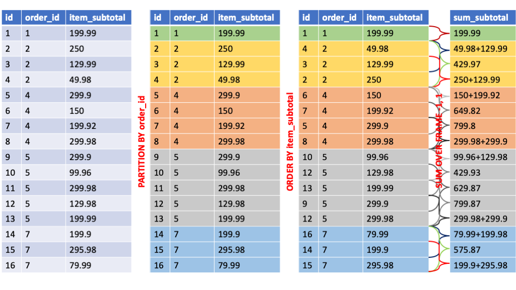
Window Functions & Ranking
An analytic function computes values over a group of rows and returns a single result for each row. This is different from an aggregate function, which returns a single result for an entire group of rows. It includes an over clause, which defines a window of rows around the row being evaluated.
Windowing specification – It includes following:
- PARTITION BY – Takes a column(s) of the table as a reference.
- ORDER BY – Specified the Order of column(s) either Ascending or Descending.
- Frame – Specified the boundary of the frame by stat and end value. The boundary either be a type of RANGE or ROW followed by PRECEDING, FOLLOWING and any value.
These three (PARTITION, ORDER BY, and Window frame) can be used alone or together.
Over
You can use OVER () to compute the average over all subtotal
hive> SELECT *, ROUND( AVG(order_item_subtotal) OVER () ,2) AS mean_subtotal FROM order_items LIMIT 5;

order_item_id order_item_order_id order_item_product_id order_item_quantity order_item_subtotal order_item_product_price mean_subtotal
1 1 957  1 299.98 299.98 199.32
2 2 1073 1 199.99 199.99 199.32
3 2 502  5 250.0  50.0   199.32
4 2 403  1 129.99 129.99 199.32
5 4 897  2 49.98  24.99  199.32
Partition By
You can use PARTITION BY clause to count order_items in each order.
hive> SELECT *, COUNT(*) OVER (PARTITION BY order_item_order_id) AS items_in_order FROM order_items ORDER BY order_item_order_id LIMIT 8;

order_item_id order_item_order_id order_item_product_id order_item_quantity order_item_subtotal order_item_product_price items_in_order
1 1 957  1 299.98 299.98 1
4 2 403  1 129.99 129.99 3
3 2 502  5 250.0  50.0   3
2 2 1073 1 199.99 199.99 3
5 4 897  2 49.98  24.99  4
8 4 1014 4 199.92 49.98  4
6 4 365  5 299.95 59.99  4
7 4 502  3 150.0  50.0   4
Order By
You can use ORDER BY clause to count order items with subtotal in descending order
hive> SELECT *, COUNT(*) OVER (ORDER BY order_item_subtotal) AS total_count FROM order_items LIMIT 5;

order_item_id order_item_order_id order_item_product_id order_item_quantity order_item_subtotal order_item_product_price total_count
575    234   775 1 9.99 9.99 172198
136754 54682 775 1 9.99 9.99 172198
70523  28198 775 1 9.99 9.99 172198
13859  5557  775 1 9.99 9.99 172198
5066   2023  775 1 9.99 9.99 172198
Order By and Partition By
You can use PARTITION BY and ORDER BY to count order_items in each order with subtotal descending order. (Wrong Version)
hive> SELECT *, COUNT(*) OVER (PARTITION BY order_item_order_id ORDER BY order_item_subtotal DESC) AS items_in_order FROM order_items ORDER BY order_item_order_id LIMIT 8;

order_item_id order_item_order_id order_item_product_id order_item_quantity order_item_subtotal order_item_product_price items_in_order
1 1 957  1 299.98 299.98 1 # order_id 1 contains 1 product
3 2 502  5 250.0  50.0   1 # wrong
2 2 1073 1 199.99 199.99 2 # wrong
4 2 403  1 129.99 129.99 3 # order_id 2 contains 3 products
8 4 1014 4 199.92 49.98  2 # wrong
7 4 502  3 150.0  50.0   3 # wrong
5 4 897  2 49.98  24.99  4 # order_id 4 contains 4 products
6 4 365  5 299.95 59.99. 1 # wrong
The result that you obtain is clearly wrong, this because of a default behavior of the ORDE BY clause, it adds a range limit to consider unbounded preceding rows and current row. Let's see how you can change it.
In windowing frame, you can define the subset of rows in which the windowing function will work. You can specify this subset using upper and lower boundary value using windowing specification. The syntax to defined windowing specification with ROW/RANGE looks like:
ROWS|RANGE BETWEEN <upper expression> AND <lower expression>
- <upper expression> can have three value: UNBOUNDED PRECEDING - it denotes window will start from the first row of the group/partition, CURRENT ROW - window will start from the current row, and <INTEGER VALUE> PRECEDING - Provide any specific row to start window.
- <lower expression> can also have three value: UNBOUNDED FOLLOWING – It means the window will end at the last row of the group/partition, CURRENT ROW – Window will end at the current row, <INTEGER VALUE> FOLLOWING – Window will end at specific row.
Order By, Partition By and Row Between
You can use PARTITION BY, ORDER BY and ROWS BETWEEN to count order_items in each order with subtotal descending order. (Good Version)
hive> SELECT *, COUNT(*) OVER (PARTITION BY order_item_order_id ORDER BY order_item_subtotal ROWS BETWEEN UNBOUNDED PRECEDING AND UNBOUNDED FOLLOWING) FROM order_items ORDER BY order_item_order_id LIMIT 8;
1 1 957  1 299.98 299.98 1
4 2 403  1 129.99 129.99 3
2 2 1073 1 199.99 199.99 3
3 2 502  5 250.0  50.0   3
7 4 502  3 150.0  50.0   4
8 4 1014 4 199.92 49.98  4
6 4 365  5 299.95 59.99  4
5 4 897  2 49.98  24.99  4
Order By, Partition By and Range Between
You can use RANGE BETWEEN to compute the mean revenue of COMPLETE and CLOSED orders in a week range, three days before order date and three days after.
hive> CREATE VIEW orders_done AS
SELECT o.order_id, o.order_customer_id, o.order_status, CAST(o.order_date AS DATE) AS order_date, T.order_revenue FROM orders AS o JOIN (SELECT order_item_order_id, round(sum(order_item_subtotal),2) AS order_revenue FROM order_items GROUP BY order_item_order_id) AS T ON T.order_item_order_id = order_id WHERE o.order_status IN ('CLOSED', 'COMPLETE');

hive> DESCRIBE orders_done;
order_id             int
order_customer_id    int
order_status         varchar(45)
order_date           date
order_revenue        double

hive> SELECT *, round(AVG(order_revenue) OVER (ORDER BY order_date RANGE BETWEEN 3 PRECEDING AND 3 FOLLOWING),2) FROM orders_done LIMIT 8;
57782 284   CLOSED   2013-07-25 1049.85 573.55
57776 5675  COMPLETE 2013-07-25 819.87  573.55
57768 3593  COMPLETE 2013-07-25 829.86  573.55
57764 1763  COMPLETE 2013-07-25 1149.92 573.55
57762 192   COMPLETE 2013-07-25 879.82  573.55
57758 10430 COMPLETE 2013-07-25 150.0   573.55
57757 6875  COMPLETE 2013-07-25 1099.87 573.55
The result shows that in the week from 2013-07-22 to 2013-07-28 the mean order revenue was 573.55 so now you can see which order revenue is over or under this mean value.
Delay and Ranking Operations
In order to maximize the utility of what you see, function windows should also be taken into account.
hive> CREATE TABLE wf_sample (id int, x int, y int);
hive> INSERT INTO TABLE wf_sample VALUES
(1, 1, 2), (2, 1, 3), (3, 1, 3), (4, 2, 1), (5, 2, 1), (6, 2, 7), (7, 1, 8), (8, 2, 8);
These are the main functions:
- LAG: the value before the current line, considering the defined order.
hive> SELECT *, LAG(id) OVER (PARTITION BY x ORDER BY y) FROM wf_sample;
id, x, y, lag
4   2  1  NULL # No id before 4 in partition
5   2  1  4
6   2  7  5
8   2  8  6
1   1  2  NULL # No id before 1 in partition
2   1  3  1
3   1  3  2
7   1  8  3
- LEAD: the value following the current line, considering the defined order.
hive> SELECT *, LEAD(id) OVER (PARTITION BY x ORDER BY y) FROM wf_sample;
id, x, y, lead
4   2  1  5
5   2  1  6
6   2  7  8
8   2  8  NULL # No id after 8 in partition
1   1  2  2
2   1  3  3
3   1  3  7
7   1  8  NULL # No id after 7 in partition
- FIRST_VALUE: the first value of the window.
hive> SELECT *, FIRST_VALUE(id) OVER (PARTITION BY x ORDER BY y) FROM wf_sample;
id, x, y, first_value
4   2  1  4
5   2  1  4
6   2  7  4
8   2  8  4
1   1  2  1
2   1  3  1
3   1  3  1
7   1  8  1
- LAST_VALUE: the last value of the window. The result may be different from what you expected, this is because of ORDER BY default.
hive> SELECT *, LAST_VALUE(id) OVER (PARTITION BY x ORDER BY y ROWS BETWEEN UNBOUNDED PRECEDING AND UNBOUNDED FOLLOWING) FROM wf_sample;
id, x, y, last_value
4   2  1  8
5   2  1  8
6   2  7  8
8   2  8  8
1   1  2  7
2   1  3  7
3   1  3  7
7   1  8  7
- ROW_NUMBER: attributes a unique value to each row, considering the defined order.
hive> SELECT *, ROW_NUMBER() OVER (PARTITION BY x ORDER BY y) FROM wf_sample;
id, x, y, row_number
4   2  1  1
5   2  1  2
6   2  7  3
8   2  8  4
1   1  2  1 # row number restarts
2   1  3  2
3   1  3  3
7   1  8  4
- RANK: attributes the same row number to the same value, leaving “holes”. It consider the defined order.
hive> SELECT *, RANK() OVER (PARTITION BY x ORDER BY y) FROM wf_sample;
id, x, y, rank
4   2  1  1
5   2  1  1
6   2  7  3 # as row number
8   2  8  4
1   1  2  1
2   1  3  2
3   1  3  2
7   1  8  4 # as row number
- DENSE_RANK: attributes the same row number to the same value, leaving no “holes”. It consider the defined order.
hive> SELECT *, DENSE_RANK() OVER (PARTITION BY x ORDER BY y) FROM wf_sample;
id, x, y, dense_rank
4   2  1  1
5   2  1  1
6   2  7  2 # keeps numeration after repetition
8   2  8  3
1   1  2  1
2   1  3  2
3   1  3  2
7   1  8  3 # keeps numeration after repetition
- CUME_DIST: calculates the relative rank of the current row within a window partition: (number of rows preceding or peer with current row) / (total rows in the window partition). In the below example you can see in (1) that there are two rows in peer because with the same rank value, the same happens in (2) but with one preceding row so at the numerator you have the value three, the total number of rows in each window is four, so al denominator the value is alway four.
hive> SELECT *, RANK() OVER (PARTITION BY x ORDER BY y),  CUME_DIST() OVER (PARTITION BY x ORDER BY y) FROM wf_sample;
id, x, y, rank, cume_dist
4   2  1  1     0.5        # 2/4 (1)
5   2  1  1     0.5        # 2/4 (1)
6   2  7  3     0.75       # 3/4
8   2  8  4     1.0        # 4/4
1   1  2  1     0.25       # 1/4
2   1  3  2     0.75       # 3/4 (2)
3   1  3  2     0.75       # 3/4 (2)
7   1  8  4     1.0        # 4/4
- PERCENT_RANK: calculates the percent rank of the current row using the following formula: (x - 1) / (number of rows in window partition - 1) where x is the rank of the current row.
hive> SELECT *, RANK() OVER (PARTITION BY x ORDER BY y), PERCENT_RANK() OVER (PARTITION BY x ORDER BY y) FROM wf_sample;
id, x, y, rank, percent_rank
4   2  1  1     0.0                    # 0/3
5   2  1  1     0.0
6   2  7  3     0.6666666666666666.    # 2/3
8   2  8  4     1.0                    # 3/3
1   1  2  1     0.0
2   1  3  2     0.3333333333333333
3   1  3  2     0.3333333333333333
7   1  8  4     1.0
- NTILE: divides the rows for each window partition, as equally as possible, into a specified number of ranked groups. It does not consider the actual value.
hive> SELECT *, NTILE(2) OVER (PARTITION BY x ORDER BY y) FROM wf_sample;
id, x, y, ntile
4   2  1  1
5   2  1  1
6   2  7  2 # group 2 in in both partitions
8   2  8  2
1   1  2  1
2   1  3  1 # same values in
3   1  3  2 # different group
7   1  8  2
You can now, using RANK and DENSE_RANK, perform ranking operations over orders_done view that I have created before. Select top five orders by date.
hive>CREATE VIEW orders_ranks AS
SELECT *, RANK() OVER (PARTITION BY order_date ORDER BY order_revenue) AS rank_revenue, DENSE_RANK() OVER (PARTITION BY order_date ORDER BY order_revenue) AS dense_rank_revenue FROM orders_done;

hive> describe orders_ranks;
order_id             int
order_customer_id    int
order_status         varchar(45)
order_date           date
order_revenue        double
rank_revenue         int
dense_rank_revenue   int
You can filter by rank_revenue if you want to select top five orders:
hive> SELECT * FROM orders_ranks WHERE rank_revenue <= 5 LIMIT 10;
191   16    CLOSED   2013-07-26 39.99  1 1
224   11938 CLOSED   2013-07-26 39.99  1 1
67419 202   COMPLETE 2013-07-26 79.98  3 2
288   8667  COMPLETE 2013-07-26 99.99  4 3
263   8026  COMPLETE 2013-07-26 100.0  5 4
534   6896  COMPLETE 2013-07-28 50.0   1 1
591   6431  COMPLETE 2013-07-28 51.99  2 2
603   6184  CLOSED   2013-07-28 129.99 3 3
526   7259  COMPLETE 2013-07-28 129.99 3 3
601   8977  COMPLETE 2013-07-28 130.0  5 4
You can filter by dense_rank_revenue if you want to select top five revenue:
hive> SELECT * FROM orders_ranks WHERE dense_rank_revenue <= 5 LIMIT 12;
191   16    CLOSED   2013-07-26 39.99  1 1
224   11938 CLOSED   2013-07-26 39.99  1 1
67419 202   COMPLETE 2013-07-26 79.98  3 2
288   8667  COMPLETE 2013-07-26 99.99  4 3
263   8026  COMPLETE 2013-07-26 100.0  5 4
57792 2743  CLOSED   2013-07-26 129.99 6 5
534   6896  COMPLETE 2013-07-28 50.0   1 1
591   6431  COMPLETE 2013-07-28 51.99  2 2
603   6184  CLOSED   2013-07-28 129.99 3 3
526   7259  COMPLETE 2013-07-28 129.99 3 3
601   8977  COMPLETE 2013-07-28 130.0  5 4
577   457   CLOSED   2013-07-28 159.98 6 5
Spark SQL APIs
You can query data in Spark SQL using SQL commands. The syntax is very similar to queries in a relational database, you can use SQL to query Hive tables directly or to query DataFrame and Dataset views. To use SQL in Spark, use the sql function in the Spark session, passing the SQL query you want to execute as a string. This returns a DataFrame, just like DataFrame transformation operations do.
If Hive and Spark are integrated, You can create DataFrames from data in Hive tables or run Spark SQL queries against it. In order to read data from Hive you can use spark.read.table API. You can prefix database name to table name.
>>> spark.sql('SHOW FUNCTIONS')You can create DataFrame from Hive table
>>> from pyspark.sql import SQLContext
>>> orders = sqlContex.table('orders')
>>> orders.count()
68883
or directly execute query Hive Tables and Views:
In this statement you can see the format of the file or files to query - in this case, Parquet - and then the path to the file or the directory containing the files. Note that the statement uses backticks to demark the file location, not single or double quotes.
SQL in Spark is not limited to querying existing data in a file or Hive table. You can also use SQL to query a DataFrame or Dataset by using temporary views. Note that the reason views are called “temporary” is that they exist just for the lifetime of your Spark session. Global views can be shared between multiple Spark sessions within a single Spark application. To create a view:
DataFrame.createTempView(view-name)
DataFrame.createOrReplaceTempView(view-name)  DataFrame.createGlobalTempView(view-name)
Here's an example of how to create and query a temporary view in Spark.
You can use the Catalog API to explore tables and manage views. The entry point for the Catalog API is spark.catalog. Functions include:
listDatabases returns a Dataset a Python list of existing databases
- setCurrentDatabase(dbname) sets the current default database for the session, it is equivalent to USE statement in SQL.
- listTables returns a a Python list of tables and views in the current database
- listColumns(tablename) returns a Python list of the columns in the specified table or view
- dropTempView(viewname) removes a temporary view
- setCurrentDatabase(dbname) sets the current default database for the session
DataFrames
DataFrames and DataSets are the primary abstractions for representing structured data in Spark, both consist of a collection of structured objects that together make up an immutable distributed set of data. DataFrames represent data into rows and columns, much like a table in a relational database system does, it allows developers to impose a structure onto a distributed collection of data. DataSets are similar but strongly-typed, so they are not available in Python.
DataFrames and DataSets use the underlying Spark APIs, so everything we said about actions, transformations, lazy evaluation, lineage, etc.. is still valid. Transformation operations create a new DataFrame as a result of performing some sort of transformation on the data in the original DataFrame. Instead the output from actions is typically either saved to a file or returned to the application’s driver process.
Some common DataFrame actions include:
- count: returns the number of rows
- first: returns the first row (synonym for head())
- take(n): returns the first n rows as an array (synonym for head(n))
- show(n): display the first n rows in tabular form (default is 20 rows)
- collect: returns all the rows in the DataFrame as an array
- write: save the data to a file or other data source
Common transformations include:
- select: only the specified columns are included
- where: only rows where the specified expression is true are included (synonym for filter)
- orderBy: rows are sorted by the specified column(s) (synonym for sort)
- join: joins two DataFrames on the specified column(s)
- limit(n): creates a new DataFrame with only the first n rows
A sequence of transformations followed by an action is a query.
Create DataFrame
To create a DataFrame from a file or table you can use spark.read API, it returns a DataFrameReader object.
format: indicates the data source type, such as csv, json, or parquet (default)
- option: specifies a key/value setting for the underlying data source
- schema: specifies a schema to use instead of inferring one from the data source
You can chain DataFrameReader settings to specify how to load data from the data source. After that, call the load method to read a file or the table method to read a Hive table.
Create from JSON
You can create a DataFrame starting from a JSON file where each line is a record, you can also use spark.read.format('json').load('data.json')it is equivalent.
Create from CSV
You can create a DataFrame starting from a CSV file, you can also use spark.read.format('csv').option('header', True).option('sep', ',').load('example.csv') it is equivalent. You can chain as many option as you want.
Create from Text
You can use spark.read.text to read text data, it can be used to read fixed length data where there is no delimiter. Default field name is value.
Create from AVRO
Since spark-avro module is external, there is no .avro API in DataFrameReader or DataFrameWriter. To load data in Avro format, you need to specify the data source option format as avro. In the below example the Avro file comes directly from the Amazon S3 Bucket. You need to provide SUBMIT_ARGS to load the jar library.
Please note that SparkFiles works only in local mode. When using SparkFiles.get in yarn mode it reports file not found exception. The problem here is that SparkFiles.get saves the file on driver, you can copy it from local file system into HDFS using the command hdfs dfs -copyFromLocal
Create from Parquet
You can create a DataFrame starting from a Parquet file. In the below example the parquest file comes directly from the Amazon S3 Bucket. You can also use spark.read.format('parquet').load(local_path) it is equivalent.
Please note that SparkFiles works only in local mode. When using SparkFiles.get in yarn mode it reports file not found exception. The problem here is that SparkFiles.get saves the file on driver, you can copy it from local file system into HDFS using the command hdfs dfs -copyFromLocal
Create from ORC
You can create a DataFrame starting from an ORC file. In the below example the ORC file comes directly from the Amazon S3 Bucket. You can also use spark.read.format('orc').load(local_path) it is equivalent.
Please note that SparkFiles works only in local mode. When using SparkFiles.get in yarn mode it reports file not found exception. The problem here is that SparkFiles.get saves the file on driver, you can copy it from local file system into HDFS using the command hdfs dfs -copyFromLocal
Create using JDBC
To read data from JDBC you need to register JDBC jar file using --packages or --jars and --driver-class-path while launching PySpark. You need to specify the table name and other properties as dict to read data from remote relational databases. You can pass a table name or query to read data using JDBC into Data Frame, also while reading data, you can define number of partitions (using numPartitions), criteria to divide data into partitions (partitionColumn, lowerBound, upperBound). Partitioning works only on numeric fields.
Creating partitions doesn't result in loss of data due to filtering. The upperBound, lowerBound along with numPartitions just defines how the partitions are to be created. The upperBound and lowerBound don't define the range (filter) for the values of the partitionColumn to be fetched.
For a given input of lowerBound (l), upperBound (u) and numPartitions (n), the partitions are created as follows:
Depending on the actual range of values of the partitionColumn, the result size of each partition can vary.
DataFrame Schema
Every DataFrame is associated with a schema that defines the names and types of the columns. The schema is defined when the DataFrame is first created. Once a schema is set, it never changes; it is immutable, just like the data in a DataFrame. You can use printSchema method to display a formatted version of the schema object.
When a new DataFrame is created by reading data from a data source, the schema is determined in one of two ways:
- It can either be inferred from the data itself,
- or you can define a schema manually
When the new DataFrame is returned as the result of a transformation on a base DataFrame, Spark calculates a new schema by analyzing the transformation.
When you create a DataFrame based on a structured data source such as a Parquet file or Hive table, the schema can be inferred from the structure of that data. Spark reads that schema from the file and uses it to create the DataFrame’s schema. Hive table schemas are part of the table’s metadata, which is stored in the Hive metastore. Spark can also attempt to infer a schema from semi-structured data in a text file such as a JSON or CSV file.
Let’s look at an example of how Spark would infer a schema from a CSV file.
The csv_data DataFrame has three columns: pcode age, which are both integer, and name, which is an string. The columns are also noted as being nullable, meaning that a row may not contain a value in that column. In the first case, without schema inference, all columns were string.
There are a couple of drawbacks to using auto-infer.
- Inferring the schema requires that Spark read every line of every file in a set of files. If you are working with a large amount of data, that will take a lot of time, hurting performance.
- The result may not match the schema you expect or need the data to have.
You can avoid both these problems by defining a schema programmatically rather than relying on Spark’s automatic schema inference.
Please note that SparkFiles works only in local mode. When using SparkFiles.get in yarn mode it reports file not found exception. The problem here is that SparkFiles.get saves the file on driver, you can copy it from local file system into HDFS using the command hdfs dfs -copyFromLocal
Defining Queries
In the DataFrames and Datasets API, the series of transformations on a starting DataFrame, followed by an action to return, save, or display the result, is known as a query. You can follow the below steps to download locally the retail_db datase an create DataFrames.
Step I. get access to retail_db database
The database retail_db is in Amazon S3 Bucket, the cluster couldn’t access to S3 because of the access restriction. You can add this policy to your EMR
{
  "Version": "2012-10-17",
  "Statement": [
    {
      "Effect": "Allow",
      "Action": "s3:*",
      "Resource": [
        "arn:aws:s3:::gmucciolo.it",
        "arn:aws:s3:::gmucciolo.it/*"
      ]
    }
  ]
}
Or you can provide you keys in spark configuration. I suggest using the previous IAM Policy where gmucciolo.it is the name of the Amazon S3 Bucket where I saved the retail_db dataset. To access another Amazon S3 Bucket you have to update the IAM Policy with the name of your Amazon S3 Bucket. The IAM Policy should be attached to the EMR cluster IAM Role. For more details how to configure AWS access see here.
Step II. create categories table
Step III. create customers table
Step IV. create departments table
Step V. create order_items table
The value of the column order_item_subtotal is equal to the product between order_item_quantity and order_item_product_price.
Step VI. create orders table
The order_date column format is 'yyyy-MM-dd HH:mm:ss'
Step VII. create products table
You can use the retail_db database to solve this problem statements:
- Get daily revenue by product considering completed and closed orders. Data need to be sorted in ascending order by date and then descending order by revenue computed for each product for each day.
- Get daily revenue by departments considering completed and closed orders in 2013 August. Data need to be sorted in ascending order by date and then descending order by revenue computed for each department for each day.
- Get the top five spending customers considering completed and closed orders.
Selection or Projection
To select data from a DataFrame you can use select or selectExpr.
- select returns a new DataFrame where there are only the selected columns
- selectExpr is the same but it let you to use SQL Expression
When you manipulate the data in a DataFrame by using Spark's build-in functions, the framework uses the operation' definition as the name for the new column. You can give a friendly name to the new column by using the alias method.
There are cases where you need to manipulate one column and select all others. It is very inconvenient to use select in this case. It is more convenient to add a new column by using withColumn, or use drop if you need all columns but one.
Filtering data
You can use where or filter to select rows that you need in order to solve the problem statement. You can also use filtering to check data quality, for example you can validate that the order_item_subtotal is equal to the product of order_item_quantity and order_item_product_price.
Exercises:
- Get all the orders which are placed on first or every month
- Get all the orders which are placed on last or every month
- Get order items where order_item_subtotal is not equal to the product of order_item_quantity and order_item_product_price
To define multiple conditions at same time you have to use brackets notation.
Here the Solutions of previous exercise.
Please note that filter and where are the same.
Joins Operations
You need to perform Join operations to combine columns from one table or more table in the retail_db database. To solve the problem statements you need to join the tables to obtain products, departments, and customers. You have to use filtered-orders from previous steps.
join(other, on=None, how=None)
Joins with another DataFrame, using the given join expression. Spark supports outer join as well.
Exercises:
- Get all orders where there are no corresponding orders_items
- Check if there are any order_items where there is no corresponding order in the orders data set. You can use Join operations to validate Foreign Keys.
Here the Solutions of previous exercise.
Aggregations
Many times you need to perform aggregations such as sum, average, minimum, maximum etc within each group. You need to first group the data and then perform aggregation, to achieve this you can use groupBy function.
Once data is grouped you can perform all supported aggregations like sum, avg, min, max etc bu using agg function. The agg function gives you the flexibility to give aliases to the derived fields.
Sorting
You can sort the data using sort and orderBy function to order data globally. If you need to perform composite sorting you can provide multiple fields. By default sort and orderBy function sort the data in ascending order but you can change the order by using desc function on a column.
Please note that sort and orderBy are the same.
If you need to sort data within a partition you can use sortWithPartitions. In this case Spark sort the data locally for each partition. You can get the current number of partitions for a DataFrame by using orders.rdd.getNumPartitions().
Spark Functions
The main package for functions in Spark is pyspark.sql.functions, you can get the whole list of built-in function and documentation using the following syntax.
Many functions in Apache Spark are similar to those in Apache Hive you already know about from the previous topic. You can import by saying from pyspark.sql import functions as F. There are functions that are not in of pyspark.sql.functions packages, in this case you can use F.expr function.
These can be categorized into
- String manipulation
- Date manipulation
- Type casting
- Expressions such as case when
Let's see some of the functions in action using orders table from retail_db database.
- F.substring(col, pos, len) - return a slice of the byte array.
- F.lower(col) - converts a string expression to lower case.
- F.date_format(date, format) - converts a date/timestamp/string to a value of string in the format specified by the date format given by the second argument.
- F.trunc(date, format) - returns date truncated to the unit specified by the format.
- F.col(col).cast(type) - convert the column col into provided type.
- F.when(condition, value_true).otherwise(value_false) - evaluates a list of conditions and returns one of multiple possible result expressions. If otherwise is not invoked, None is returned for unmatched conditions. You can chain "when" clause many times.
- F.coalesce(*cols) - returns the first column that is not null.
- F.udf(f=None, returnType=StringType) - creates a user defined function (UDF).
Window Package
You can use APIs in Window Package to perform operations like aggregations, ranking, and windowing functions within each group using APIs such as over, partitionBy, etc. The Window Functions work over a group of rows, also known as a window, and let you assign a value for each row in the source database as result of an aggregation on the window. Instead, groupBy operation results in a reduction of rows and it put limitation on columns selection. For more details how to configure AWS access see here.
An analytic function computes values over a group of rows and returns a single result for each row. This is different from an aggregate function, which returns a single result for an entire group of rows. It includes an over clause, which defines a window of rows around the row being evaluated.
For example, using the retail_db, if you want to perform a comparison between each product's price and the category total, you have two options.
- groupBy and Join operations. This solution is very expensive.
- Window Package
In order to use Window function you need to import classes from pyspark.sql.window, it contains Window and WindowSpec. Window have APIs such as partitionBy, orderBy etc. There APIs return WindowSpec object that you can pass to over function such as rank(), dense_rank(), sum().
The Window class has many methods you can use to define a WindowSpec object.
partitionBy(*cols)
You can use this to define the logic to use in partitioning, it groups rows in a window. Many functions like sum(), avg() require partition definition in WindowSpec. When you use it with orderBy it generates partitions on which performs ordering.
Given a DataFrame containing the following data:
+------+
|column|
+------+
| 10   | index = 0
| 20   | index = 1
| 30   | index = 2
| 31   | index = 3
+------+
You can create a WindowSpec with the frame boundaries defined, from start to end, both are inclusive.
rangeBetween(start, end)
This function lets you create a WindowSpec with the frame boundaries, where start and end parameters are related to the values in the column. Both start and end are relative to current row.
The range-based boundary uses the actual value of the ORDER BY expression(s).
ORDER BY column RANGE BETWEEN 2 PRECEDING AND CURRENT ROW
Given x=31 the current row's value, the function takes all rows where value is between x-2 and x, so using the above data the function returns [30, 31].
rowsBetween(start, end)
This function lets you create a WindowSpec with the frame boundaries, where start and end parameters are related to the index of the row. It doesn't care about the exact values. It cares only about the order of rows, and takes fixed number of preceding and following rows when computing the window. Both start and end are relative to current row. For example, 0 means "current row", while -1 means one before the current row, and 5 means the five after the current row.
The row-based boundary uses the position of the row within the partition.
ORDER BY column ROWS BETWEEN 2 PRECEDING AND CURRENT ROW
Given y=3 the value of the current row index, the function takes all rows where index is between y-2 and y, so using the above data the function returns [20, 30, 31].
You can use Window.unboundedPreceding, Window.unboundedFollowing, and Window.currentRow to specify special boundary values, rather than using integral values directly. A range-based boundary is based on the actual value of the ORDER BY expression(s).
orderBy(*cols)
You can use this to define the logic to use to order data. Many functions like rank(), dense_rank() require order definition in WindowSpec. When you use it with partitionBy it performs sort locally.
The orderBy function has by default a range limit with the following definition
.rangeBetween(Window.unboundedPreceding, Window.currentRow)
if you want a window that spans over the whole partition you have to add this definition
.rowBetween(Window.unboundedPreceding, Window.unboundedFollowing)
Let's have some examples about:
- sum, avg, min, max
- rank, dense_rank, row_number
- lead, lag
Sum, Avg, Min, Max
For each Category compute the Category Total - The sum over Order Item Subtotal in a Category, Category Avg - The mean over Order Item Subtotal in a Category, Category Min - The min over Order Item Subtotal in a Category, Category Max - The max over Order Item Subtotal in a Category, and the ratio between the order item subtotal and the Category Total.
You can use this syntax: F.sum(column).over(window_spec).
Rank, Dense_rank, Row_number
You can use these functions to perform ranking operation. The rank function, as well as dense_rank and row_number, does not takes any parameters. It is mandatory to provide orderBy and you cannot change frame specification.
Please, consider these problem statements:
- Get top N customers, consider spendings of closed and completed orders, including spending repetitions.
- Get top N products, consider days' revenue for closed and completed orders.
Get top N customers
You have to use dense_rank in this case because of cam have some spending repetitions. The difference between rank and dense_rank is that dense_rank leaves no gaps in ranking sequence when there are ties. That is, if there had three customers tie for second place, you would say that all three were in second place and that the next person came in third.
Get top N products
In this case you want to perform ranking over partition, so you need to specify partitionBy in your frame definition.
Lead, Lag
The LAG function has the ability to fetch data from a previous row, while LEAD fetches data from a subsequent row. This is by default, but you can pass the row number's offset as parameter.
Please, consider this problem statement:
- For each product calculate which is the next most expensive for each category and the price difference between the two.
Bonus Example
- For each product in each category calculate the next price. Compute also the difference between the current product's price and the next price. Skip price replications.
Save DataFrame
Previously you used the Spark API to solve the following problem statements:
- Get daily revenue by product considering completed and closed orders. Data need to be sorted in ascending order by date and then descending order by revenue computed for each product for each day.
- Get daily revenue by departments considering completed and closed orders in 2013 August. Data need to be sorted in ascending order by date and then descending order by revenue computed for each department for each day.
- Get the top five spending customers considering completed and closed orders.
Save data into HDFS data as text file
You can save the data delimited by "|" using RDDs transformations.
Save data into HDFS as CSV file
To provide a header to CSV file you have to pass header=True, there are also other options you can use to control escape, nullValue, lineSep, etc.
Save data into HDFS data as orc file
When you save your data, you can reduce the number of partitions by using coalesce, this generates many files in number equal to the value passed as argument to the method. In this particular example, you can see also partitionBy - that gives you the possibility to partition the result by column value - and compression - used to reduce the size of the final output - that are not peculiar to the orc method, you can use them with most of the saving formats. Here you see how to save data to orc file.
Save data into HDFS as parquet file
In this example I save the parquet file using again partitionBy and compression. The mode 'overwrite' will delete all data in the path before the saving operation.
Save data into HDFS as JSON file
The result of JSON method is a file with many lines, one for each record in the source DataFrame.
Save data into HDFS as AVRO
Usually AVRO is a 3rd party plugin, but Cloudera clusters get by it default. In this example you can see how you can load AVRO jar.
Save data into Hive Table
If Spark and Hive are integrated you can save your data as table. You can provide the path and the format of the generated files.
Submit Spark Application
You can develop a Spark Application and run it on the cluster. Later in the lesson, I show you how to define the application.properties file with contains all required input path and output path along with execution mode. You have to create the SparkContext - the spark-submit command does not provide it for you - develop your application as always, ship it to the cluster and run.
$ tree spark_application
spark_application
└── src
    ├── python
    │   └── main.py
    └── resources
        └── application.properties
The application configuration contains all the information about execution mode, input and output directory. This file is very useful, you can use it to run your application both in local and on cluster.
The main.py file contains the application's code. When submitting your code you need to provide env parameter, then the config parser selects the properties.
Now you can submit your application. You can use spark-submit to run it locally
bash>spark-submit src/python/main.py dev
or provide additional parameters to run it on cluster.
bash>spark-submit src/python/main.py prod --num-executors 5 --executor-memory 2700M --executor-cores 2
You can also select the number of executors by understanding the properties of your dataset. For example, you can obtain dataset size using:
bash> hdfs dfs -ls -h <path>
Also, you can check the number of blocks
bash> hdfs fsck <path>
...
Total blocks (validated): 7 (avg. block size 241528285 B)
...
In this case, you need to use seven or fewer executors. Let's keep using five executors. The block size defines the number of blocks. You can change the block size using:
bash> hdfs dfs -D dfs.blocksize=268435456 -put <local_path> <hdfs_path>
After that you can start implementing your application.
If your data is in CSV format, it might be convenient to read it using spark.read.csv, but in this case, you have to deal with Row objects if you need to use some Spark Core APIs.
>>> df = spark.read.csv('orders.csv', header=True)
>>> rdd = df.select('order_date', 'order_customer_id').rdd.take(2)
[Row(Primary Type='DECEPTIVE PRACTICE', substring(Date, 1, 10)='01/01/2001'), Row(Primary Type='CRIM SEXUAL ASSAULT', substring(Date, 1, 10)='10/08/2017')]
You can use the map function to cast the Row Object into a list.
>>> rdd = df.select('order_date', 'order_customer_id').rdd.map(list).take(2)
[['DECEPTIVE PRACTICE', '01/01/2001'], ['CRIM SEXUAL ASSAULT', '10/08/2017']]
Since, because of aggregations, the size of the final result is less than the input file, you may be required to reduce the number of partitions to create fewer files.
>>> codec = "org.apache.hadoop.io.compress.GzipCodec"
>>> result.coalesce(2).saveAsTextFile('result/path', codec)
You can use coalesce to decrease the files count.

Comments